
What's Inside
Concept 1
SQL vs NoSQL
Two Philosophies of Data Storage
Every system needs to store data, and your choice of database fundamentally shapes your architecture. SQL databases (relational) and NoSQL databases (non-relational) represent two different philosophies about how data should be organized, queried, and scaled. Neither is universally better — each excels in different scenarios. Understanding when to use which is one of the most important skills in system design.
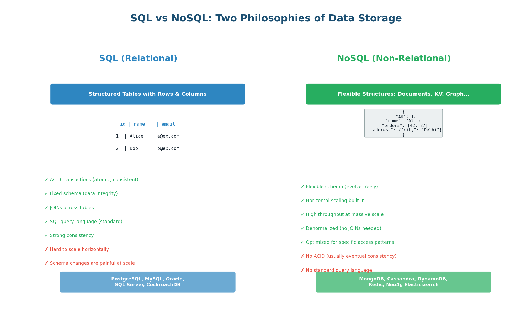
SQL (Relational) Databases
SQL databases store data in tables with predefined columns and data types. Every row in a table has the same structure (schema). Tables are related to each other through foreign keys, and you can combine data from multiple tables using JOINs. The SQL query language is standardized and powerful, supporting complex queries, aggregations, and transactions.
ACID Transactions: SQL databases guarantee Atomicity (all or nothing), Consistency (valid states only), Isolation (transactions do not interfere), and Durability (committed data is permanent). When you transfer $100 between bank accounts, ACID ensures the money leaves one account and arrives in the other — never lost, never duplicated.
Fixed Schema: You define the structure upfront (columns, types, constraints). This enforces data integrity: you cannot store a string in an integer column. The trade-off is that schema changes (ALTER TABLE) on tables with billions of rows can take hours and require downtime.
JOINs: Data is normalized (split across multiple tables to avoid duplication). A user's orders are in the orders table, not embedded in the users table. You JOIN them at query time: SELECT * FROM users JOIN orders ON users.id = orders.user_id. This keeps data consistent but JOINs become expensive at massive scale.
Use SQL for: financial systems (payments, banking), e-commerce (orders, inventory), user authentication, any domain requiring strong consistency and complex relationships. Examples: PostgreSQL (most popular choice), MySQL, Amazon Aurora. The rule of thumb: if you would naturally draw an ER diagram for your data, use SQL.
NoSQL (Non-Relational) Databases
NoSQL databases abandon the relational model in favor of simpler, more scalable data structures. Instead of tables with fixed schemas, NoSQL uses flexible formats: documents (JSON), key-value pairs, wide columns, or graphs. NoSQL databases are designed to scale horizontally (adding more machines) rather than vertically (bigger machine), and they typically sacrifice some consistency guarantees in exchange for performance and availability.
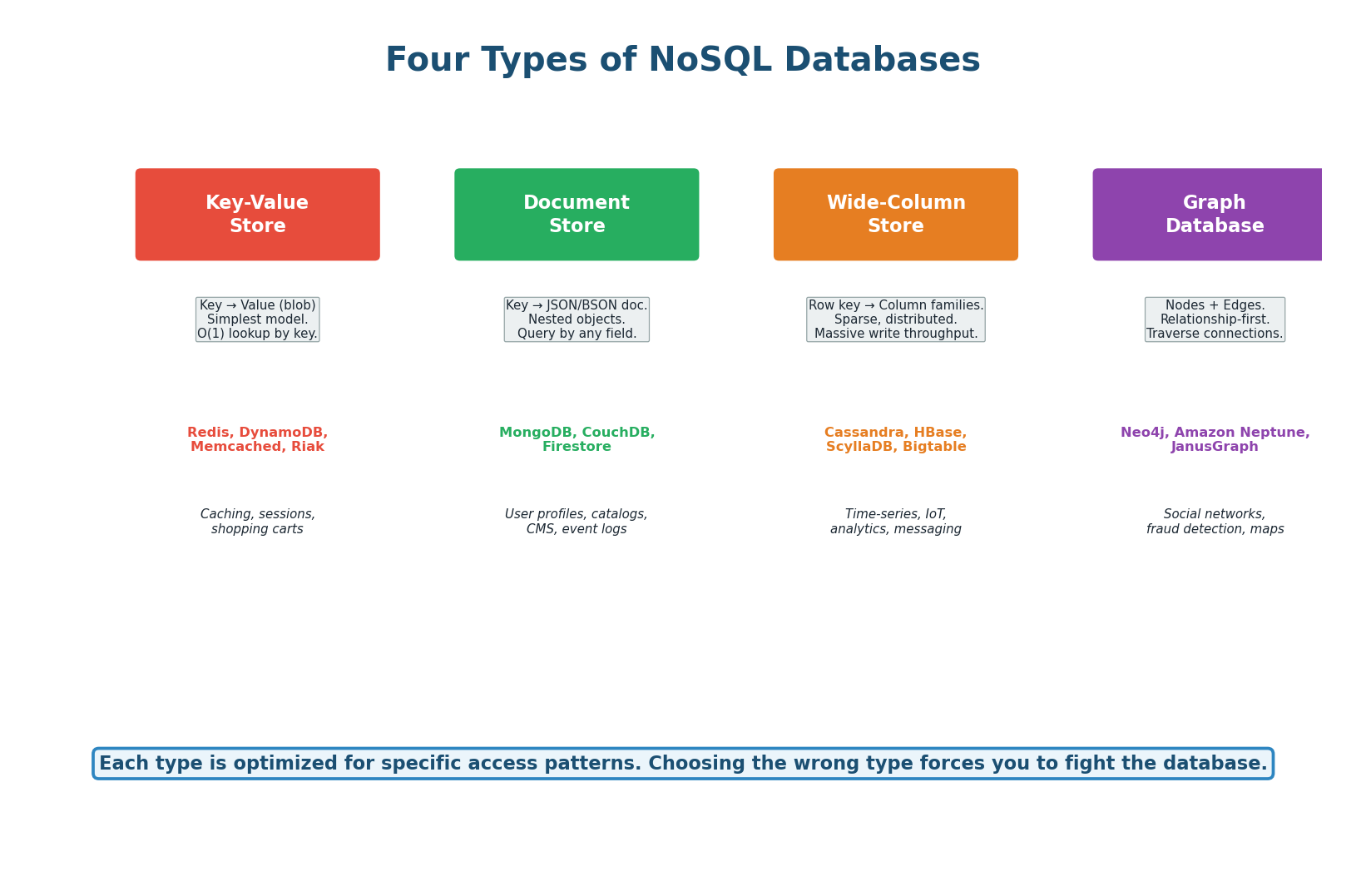
Key-Value Stores (Redis, DynamoDB): The simplest model — every piece of data is stored as a key-value pair. The key is a unique identifier, and the value can be anything (string, number, JSON blob, binary). Lookups are O(1) by key. You cannot query by value (no "find all users named Alice"). Think of it as a giant hash map. Use for: caching, sessions, shopping carts, rate limit counters, leaderboards.
Document Stores (MongoDB, CouchDB): Store data as JSON (or BSON) documents. Each document can have a different structure (flexible schema). You can nest objects and arrays inside documents. You can query by any field, not just the key. Think of it as key-value where the value is always a queryable JSON document. Use for: user profiles, product catalogs, content management, event logs.
Wide-Column Stores (Cassandra, HBase): Data is organized by row key, column family, and column name. Each row can have different columns (sparse storage). Optimized for massive write throughput and time-series data. Think of it as a two-dimensional key-value store: row key + column name = value. Use for: IoT sensor data, time-series metrics, messaging (Discord uses Cassandra for trillions of messages), analytics.
Graph Databases (Neo4j, Neptune): Store data as nodes (entities) and edges (relationships). Optimized for traversing connections: "Find all friends of friends who like this movie." Relational databases can do this with JOINs, but performance degrades rapidly as relationship depth increases. Graph databases maintain near-constant-time traversal regardless of total data size. Use for: social networks, recommendation engines, fraud detection.
| Aspect | SQL | NoSQL |
|---|---|---|
| Schema | Fixed (predefined columns) | Flexible (per-document) |
| Transactions | Full ACID | Usually eventual consistency (BASE) |
| Query language | Standardized SQL | Database-specific APIs |
| Scaling | Vertical (bigger machine) | Horizontal (more machines) |
| JOINs | Yes (powerful) | No (denormalize instead) |
| Best for | Structured data, complex queries, transactions | Flexible data, massive scale, simple access patterns |
| Examples | PostgreSQL, MySQL, Aurora | Redis, MongoDB, Cassandra, DynamoDB |
Decision Guide: Which to Choose?
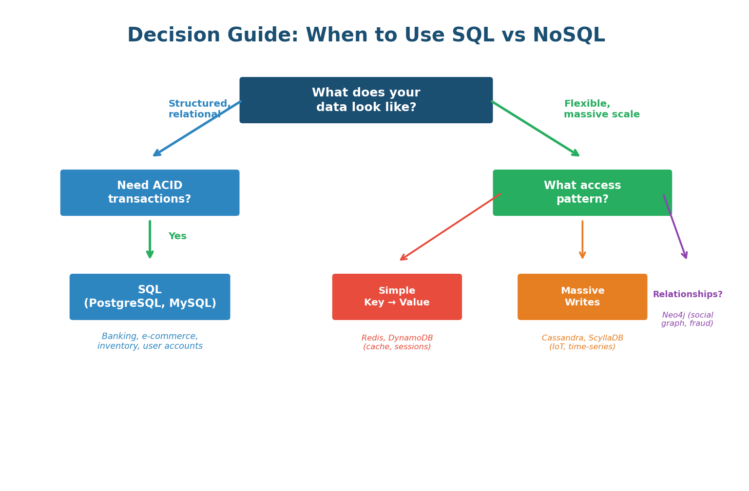
The decision framework: start with SQL. If you hit a specific limitation (schema flexibility needed, write volume exceeds one machine, data model maps naturally to key-value or graph), then consider the specific NoSQL type that fits. Most production systems use polyglot persistence — SQL for core transactional data (orders, users) and NoSQL for specific use cases (Redis for caching, Elasticsearch for search, Cassandra for time-series).
Interviewers hear "NoSQL scales better than SQL" all the time — and it's an oversimplification that signals shallow understanding. The correct answer: "SQL scales well vertically and with read replicas. NoSQL scales horizontally for write-heavy workloads. For most systems at most scales, PostgreSQL with proper indexing and replication is more than sufficient. I would choose NoSQL only when I have a specific need it uniquely addresses." This shows nuance.
Concept 2
Database Indexing
Why Indexes Are Critical
Without an index, every query requires scanning every row in the table (a full table scan). On a table with 10 million rows, this means reading 10 million rows to find one. With a B-Tree index, the same query reads approximately 24 rows (log₂ of 10 million). That is a 400,000x speedup. Indexes are the single most impactful performance optimization for any database-backed system.
Think of a book's index: instead of reading the entire book to find "consistent hashing," you look up "C" in the index, find "consistent hashing: page 147," and go directly to page 147. A database index works the same way — it maintains a sorted data structure (B-Tree) that points directly to the rows matching your query.
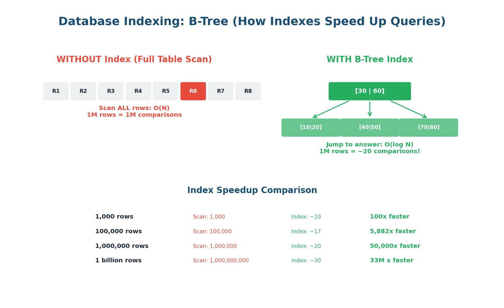
How B-Tree Indexes Work
A B-Tree is a balanced tree data structure where each node contains multiple keys and pointers. The root node divides the key space into ranges, and each range points to a child node that further subdivides. The leaf nodes contain pointers to the actual rows in the table. To find a value, you start at the root and follow the correct branch at each level — typically 3–4 levels for even billions of rows.
When you run SELECT * FROM users WHERE email = 'alice@example.com', the database checks if there is an index on the email column. If yes, it traverses the B-Tree (3–4 comparisons), finds the pointer to Alice's row, and reads it directly. If no index, it reads every row in the table until it finds a match. For 10 million users, that is the difference between 4 disk reads and 10 million disk reads.
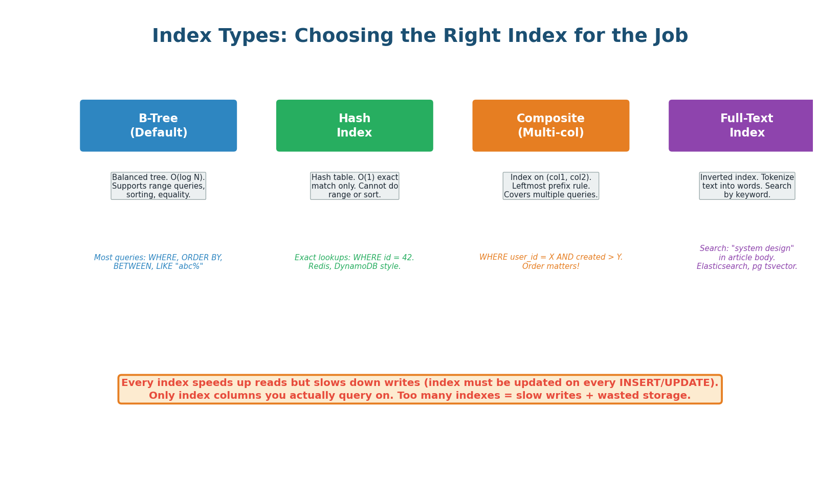
Every index speeds up reads but slows down writes. On every INSERT, UPDATE, or DELETE, the database must update all indexes on that table. A table with 10 indexes is 10x more expensive to write to than one with no indexes. Index the columns you actually query on. Never add indexes "just in case." Over-indexing is a real production problem — it causes slow writes and wastes disk space.
Index Types
| Index Type | Structure | Best For | Limitation |
|---|---|---|---|
| B-Tree | Balanced tree | Equality and range queries (=, <, >, BETWEEN, LIKE 'abc%') | Slower than Hash for pure equality |
| Hash | Hash table | Exact equality only (WHERE id = 42) | Cannot do range queries |
| Composite | B-Tree on multiple columns | Queries filtering on multiple columns | Leftmost prefix rule (see below) |
| Full-Text | Inverted index | Text search (LIKE '%word%', MATCH AGAINST) | Storage overhead; separate from B-Tree |
| Partial | B-Tree on filtered rows | Index only a subset (e.g., active users) | Only helps queries with the same filter |
Composite Indexes and the Leftmost Prefix Rule: A composite index on (user_id, created_at) can be used for queries on user_id alone OR on (user_id AND created_at). It cannot be used for queries on created_at alone — the database can only use the index starting from the leftmost column. This is called the leftmost prefix rule. If you frequently query by created_at alone, you need a separate index on created_at.
When designing a system, interviewers love when you mention indexes proactively: "For the messages table I would index on (conversation_id, created_at) — a composite index. This supports the primary query pattern 'get the last 50 messages in conversation X' since we filter by conversation_id and sort by created_at." Demonstrating index design shows you think beyond schemas to query performance.
Concept 3
Database Replication
Why Replicate: Availability, Durability, and Read Scaling
A single database server is a single point of failure. If it crashes, your entire application goes down. If its disk dies, your data is lost. Replication solves both problems by maintaining identical copies of your data on multiple servers. If the primary server fails, a replica takes over. If a disk dies, the data exists on other machines. Replication also enables read scaling: instead of one server handling all read queries, you can distribute reads across multiple replicas.
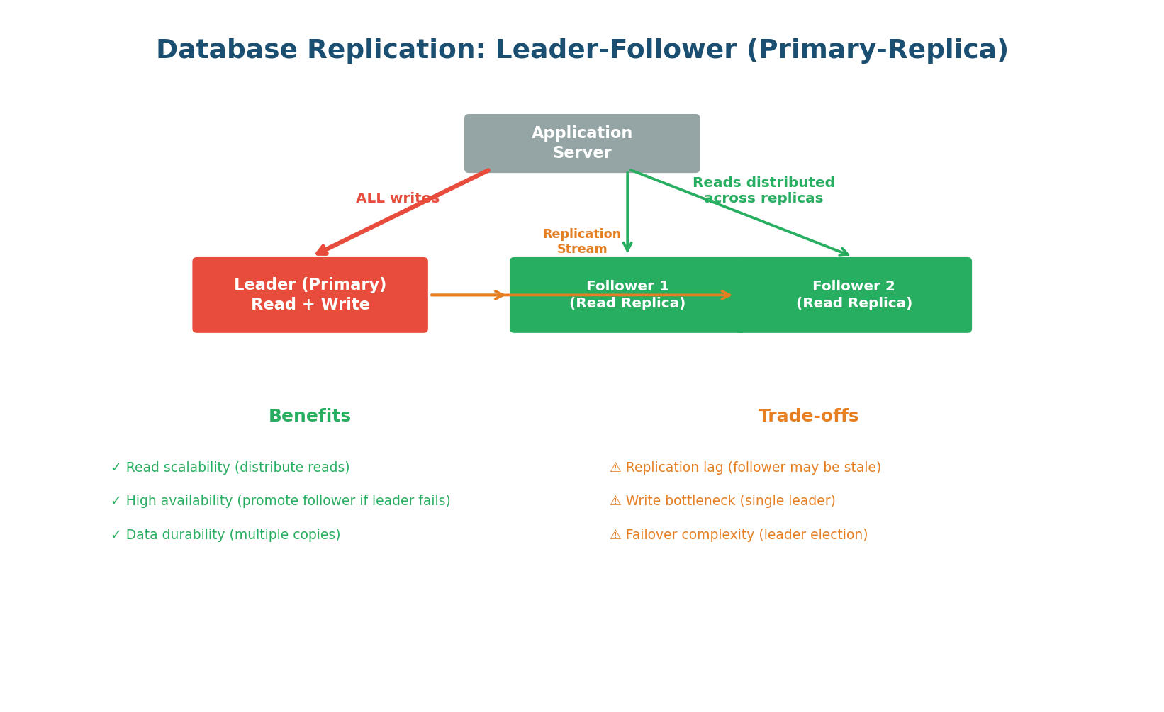
Leader-Follower (Primary-Replica) Replication
The most common replication topology. One server is designated as the leader (primary). All write operations go exclusively to the leader. The leader then streams the changes to one or more followers (replicas) via a replication log. Followers are read-only copies. Read queries can go to any follower, distributing the read load.
Write path: Client → Leader → Write to WAL (Write-Ahead Log) → Apply to data → Stream WAL to followers. The leader is the single source of truth for writes.
Read path: Client → Any follower (or leader). With 3 followers handling reads, you have 3x the read capacity. For a system with 90% reads and 10% writes, this is transformative.
Failover: If the leader crashes, one follower is promoted to be the new leader (leader election). This can be automatic (managed databases like AWS RDS, Aurora) or manual. During promotion, there is a brief window where writes are rejected. The promoted follower becomes the new leader and starts accepting writes.
Replication is not instantaneous. Between a write on the leader and its appearance on a follower, there is replication lag — typically 1–100ms in healthy systems, but potentially seconds during high load or network issues. This means a user who writes data and immediately reads from a follower may not see their own write. The solution: route critical reads (e.g., "show me my just-submitted order") to the leader, and route non-critical reads (e.g., product listings, analytics) to followers.
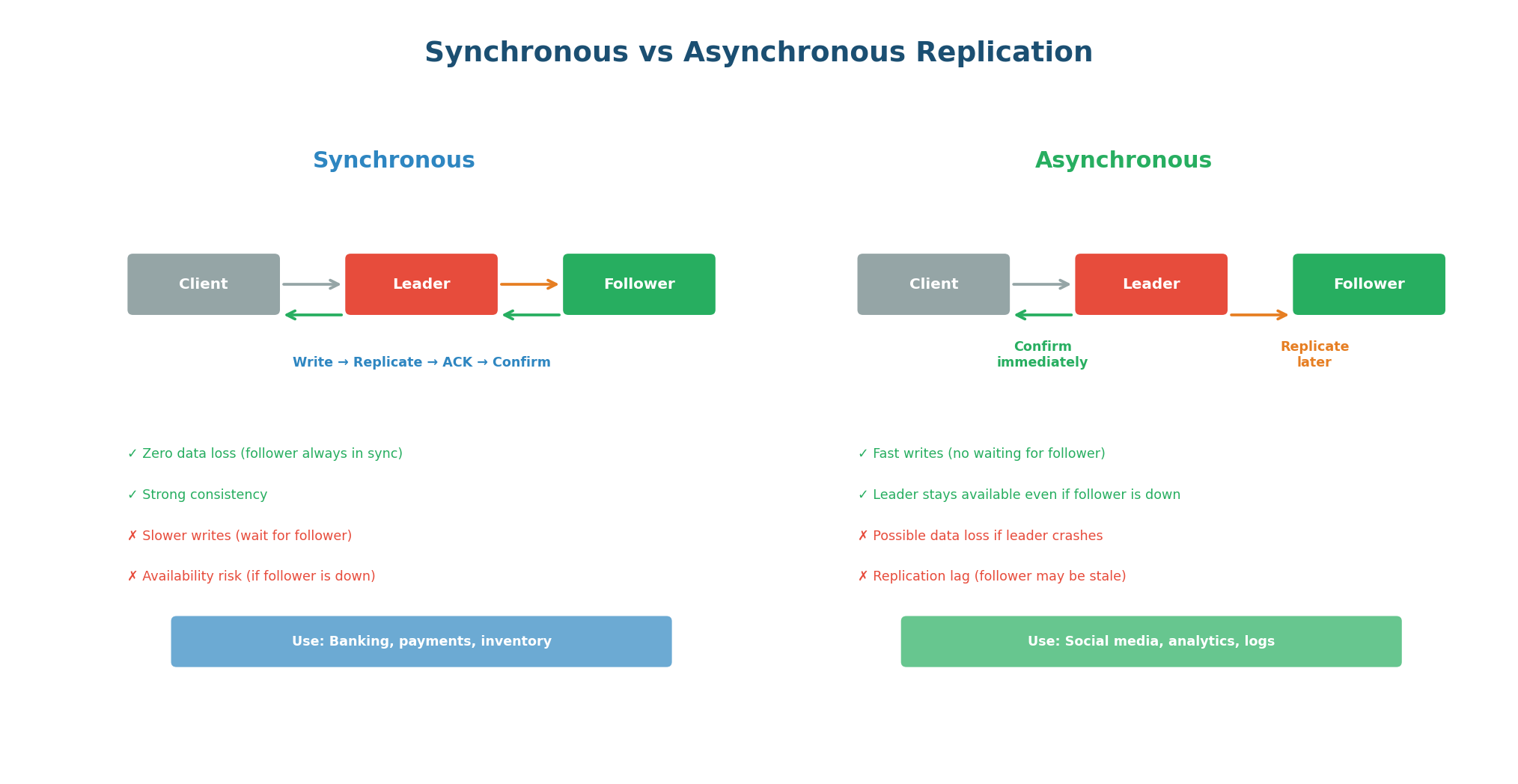
Synchronous vs Asynchronous Replication
| Mode | How It Works | Data Safety | Write Latency | Use Case |
|---|---|---|---|---|
| Synchronous | Leader waits for follower ACK before confirming write to client | Zero data loss (2 copies minimum) | Higher (adds follower RTT) | Financial transactions, critical data |
| Asynchronous | Leader confirms write immediately; follower catches up later | Possible data loss if leader crashes before replicating | Low (leader RTT only) | High-throughput writes, analytics |
| Semi-synchronous | One follower is synchronous; rest are async | At least 2 copies before ACK | Moderate | Best of both (practical default) |
Semi-synchronous is the practical compromise: one follower is synchronous (guarantees at least one copy exists before confirming), and additional followers are asynchronous (for read scaling without impacting write latency). PostgreSQL and MySQL both support this mode. This gives you data durability (two copies before confirming) with reasonable write performance.
In every system design answer that involves a database, include replication: "I will use a primary PostgreSQL instance with 2 read replicas. All writes go to the primary. Read-heavy endpoints like product search and user profile reads go to the replicas, giving 3x read capacity. The primary has synchronous replication to one replica for durability. If the primary fails, the synchronous replica is promoted automatically."
When a Single Database Is Not Enough
Replication scales reads, but it does not scale writes. Every write still goes to a single leader. When your write volume exceeds what one machine can handle — or your data exceeds what fits on one machine's disk — you need sharding. Sharding splits your data across multiple independent database instances (shards), each holding a subset of the total data. Each shard handles reads and writes for its own subset.
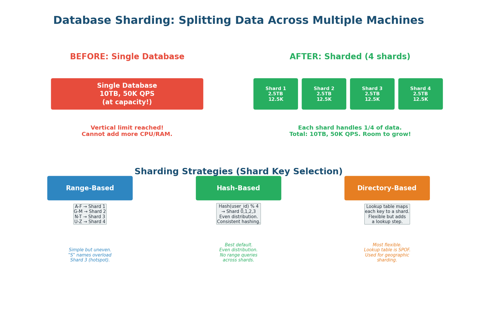
Choosing a Shard Key
The shard key determines which shard holds each piece of data. This is the most critical decision in sharding because a bad shard key causes hotspots (one shard overwhelmed while others sit idle) and makes cross-shard queries expensive. The ideal shard key has high cardinality (many unique values), even distribution (each shard gets roughly equal data), and aligns with your query patterns (queries rarely need to span multiple shards).
Hash-Based Sharding (Recommended Default): Apply a hash function to the shard key (e.g., user_id) and use modulo to select the shard: shard = hash(user_id) % num_shards. This produces even distribution regardless of the key's natural distribution. The downside: range queries (WHERE user_id BETWEEN 1000 AND 2000) must scatter across all shards because hashing destroys natural ordering. Use consistent hashing to minimize data movement when adding/removing shards.
Range-Based Sharding: Assign contiguous ranges of the shard key to each shard: users with IDs 1–100K go to Shard 1, 100K–200K go to Shard 2. This preserves range query efficiency (all users in a range are on the same shard) but can create hotspots: if new users get incrementing IDs, the latest shard receives all new writes while older shards are nearly idle.
Directory-Based Sharding: A separate lookup service maintains a mapping from each key to its shard. The most flexible approach (any key can be on any shard), but the lookup service itself becomes a single point of failure and a bottleneck. Used for geographic sharding: users in India → Mumbai shard, users in the US → Virginia shard. The directory is cached to avoid the lookup bottleneck.
Sharding Challenges
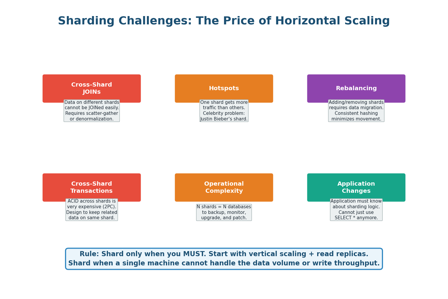
- Cross-Shard Queries: A query spanning multiple shards (e.g., "top 10 users by order count globally") must be sent to all shards, results gathered and merged. This is expensive and slow. Design your shard key so the most frequent queries stay within a single shard.
- Cross-Shard Transactions: ACID transactions across shards require distributed transaction protocols (two-phase commit), which are complex, slow, and prone to failure. Avoid cross-shard transactions wherever possible by co-locating related data on the same shard.
- Rebalancing: When you add a new shard, data must be moved from existing shards to the new one. Without consistent hashing, this can mean moving nearly all your data. With consistent hashing, only ~1/N of data moves.
- Schema Changes: With N shards, every
ALTER TABLEmust be run on every shard. This multiplies operational complexity by N. - Hotspots: If your access pattern is not uniform (e.g., celebrity users getting 1000x more traffic), even hash-based sharding can create hotspots. Mitigate with virtual nodes or by adding a random suffix to the shard key for ultra-hot rows.
The Database Scaling Ladder
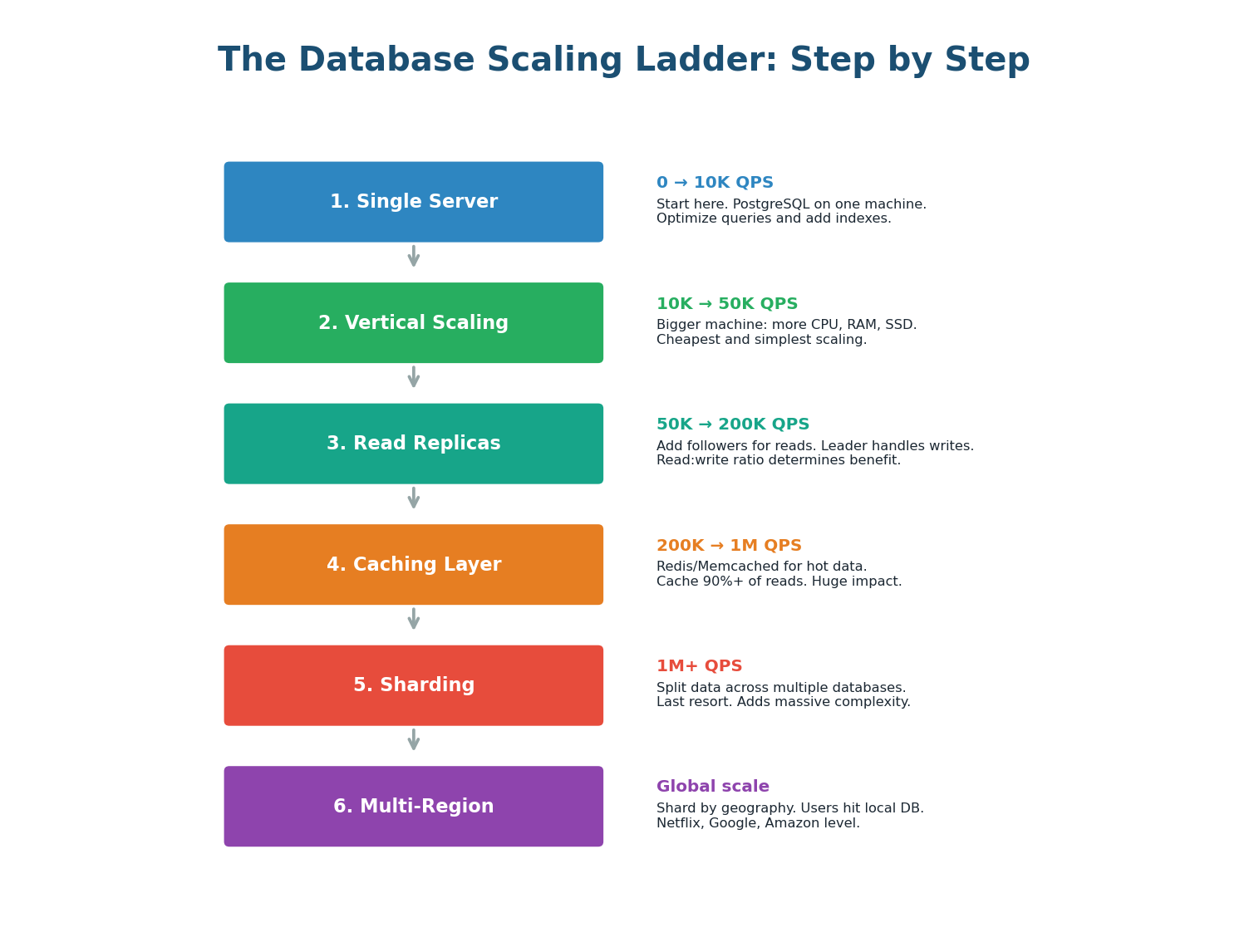
Database scaling is not a single decision; it is a sequence of steps you take as your system grows. Each step adds complexity, so you should only move to the next step when the current one is insufficient.
| Step | Technique | What It Solves | Added Complexity |
|---|---|---|---|
| 1 | Single server | Starting point | None |
| 2 | Vertical scaling | Higher CPU/RAM/disk | Low (hardware only) |
| 3 | Read replicas | Read throughput + HA | Replication lag handling |
| 4 | Caching (Redis) | Reduce DB load | Cache invalidation logic |
| 5 | Sharding | Write throughput + data volume | High (cross-shard queries, rebalancing) |
| 6 | Global distribution | Multi-region latency | Very high (geo-replication, conflict resolution) |
Sharding is the nuclear option of database scaling. Before sharding, exhaust every other option: proper indexing, query optimization, connection pooling, vertical scaling, read replicas, and caching. Instagram ran on a single PostgreSQL server until it was acquired by Facebook with over 30 million users. Most systems never need sharding. If an interviewer asks when to shard: "Only when a single node with replicas cannot handle write throughput or data volume — typically hundreds of millions of rows or thousands of writes per second."
Pre-Class Summary
The Four Pillars of Data Storage
SQL vs NoSQL: SQL for structured data with transactions (banking, e-commerce). NoSQL for flexible schema at massive scale (caching, IoT, social). Most real systems use both — polyglot persistence is the norm, not the exception.
Indexing: B-Tree indexes turn O(N) full table scans into O(log N) lookups. Every index speeds up reads but slows down writes. Index the columns you actually query on. Composite indexes follow the leftmost prefix rule.
Replication: Leader-follower replication provides read scaling, high availability, and data durability. Synchronous replication gives zero data loss but slower writes. Asynchronous gives fast writes but possible replication lag. Semi-synchronous is the practical default.
Sharding: Splits data across multiple machines for write scaling and large data volumes. Choose a shard key that distributes data evenly and aligns with your access pattern. Hash-based sharding is the best default. Shard only as a last resort — the operational complexity is enormous.
Want to Land at Google, Microsoft or Apple?
Watch Pranjal Jain's free 30-min training — the exact GROW Strategy that helped 1,572+ engineers go from TCS/Infosys to top product companies with a 3–5X salary hike.