
What's Inside
Topic 1
Database Trade-offs
The Fundamental Triangle: Reads vs Writes vs Storage
Every database makes trade-offs between three competing goals: read performance (how fast can you query?), write performance (how fast can you insert/update?), and storage efficiency (how much disk space does it use?). Optimizing for one inevitably costs another. Understanding this triangle is essential for choosing the right database and the right configuration for your workload.
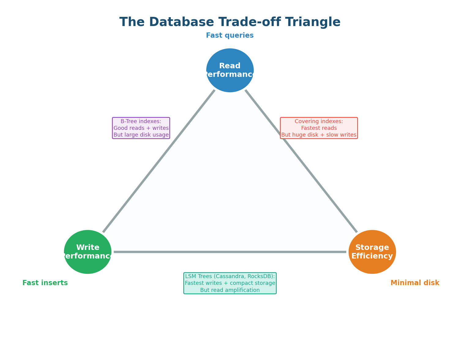
Adding more indexes makes reads faster but makes writes slower (each index must be updated on every write) and uses more disk. Denormalizing data (storing pre-computed JOINs) makes reads faster but doubles storage and makes writes more complex. Using an append-only storage engine (LSM-Tree) makes writes blazingly fast but can slow down reads. There is no free lunch — every optimization is a trade-off.
B-Tree vs LSM-Tree: The Storage Engine Choice
Under the hood, every database uses a storage engine that determines how data is physically written to and read from disk. The two dominant architectures are B-Tree (used by PostgreSQL, MySQL, Oracle) and LSM-Tree (used by Cassandra, RocksDB, LevelDB, ScyllaDB). This is the most consequential low-level trade-off in database design.
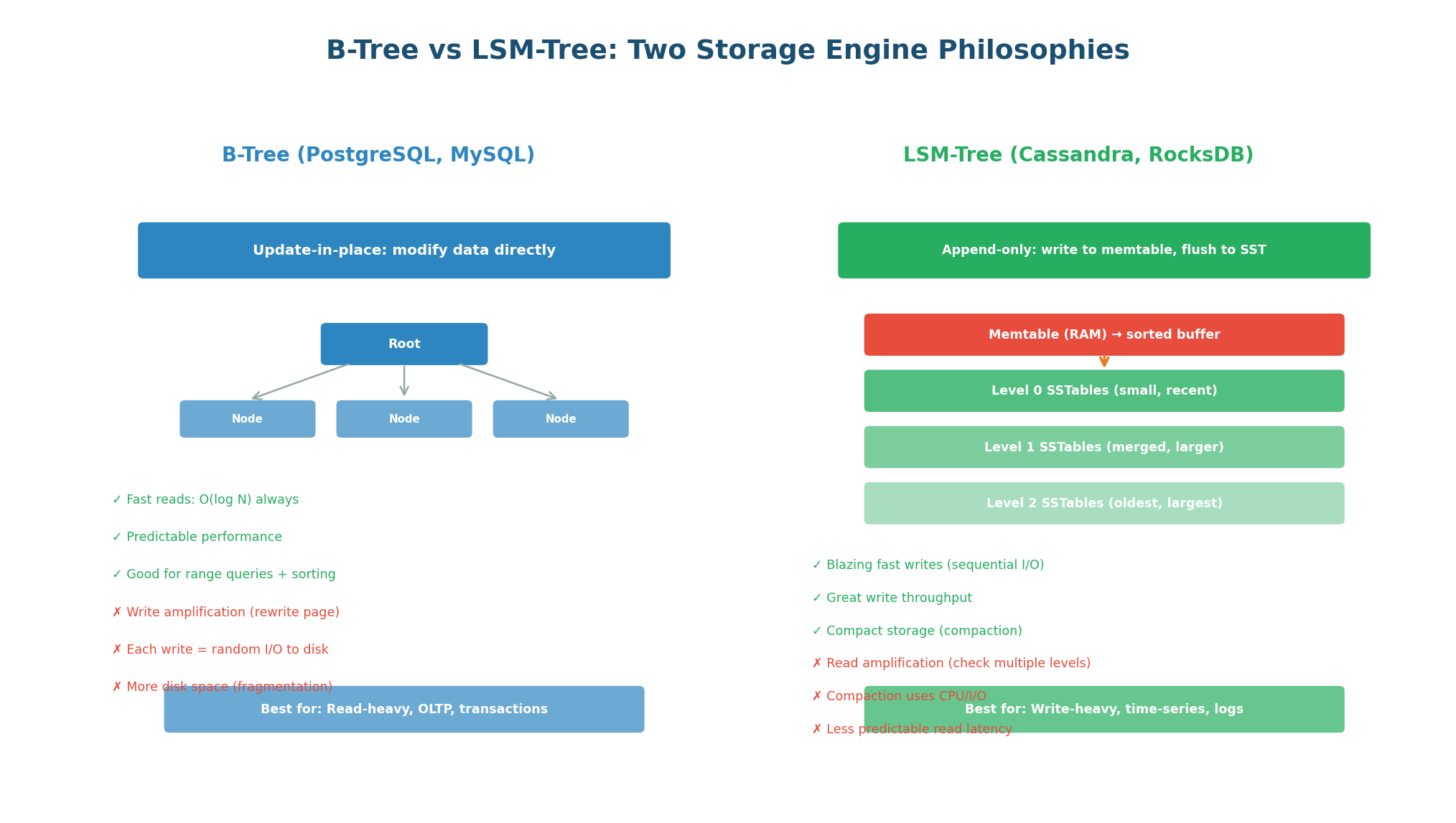
B-Tree: Update-in-Place. B-Trees store data in fixed-size pages (typically 4–16 KB) organized in a balanced tree. When you write data, the B-Tree finds the correct page and updates it in place. Reads are always O(log N) because you traverse the tree from root to leaf. The write path involves random I/O (jumping to the correct page on disk), which is slower than sequential I/O. B-Trees also suffer from write amplification: a single logical write can trigger multiple page rewrites for balancing and COW (copy-on-write).
Best for: Read-heavy workloads (OLTP), transaction processing, systems where reads vastly outnumber writes. PostgreSQL, MySQL InnoDB, and most traditional RDBMS use B-Trees.
LSM-Tree: Append-Only. LSM-Trees (Log-Structured Merge Trees) never update data in place. Instead, writes go to an in-memory buffer (memtable). When the memtable fills up, it is flushed to disk as an immutable sorted file (SSTable). Periodically, SSTables are merged (compacted) to remove duplicates and reclaim space. Because writes are always sequential (appending to the memtable, flushing sorted data), write throughput is 5–10x higher than B-Trees on the same hardware.
The read trade-off: To read a key, the LSM-Tree must check the memtable, then Level 0 SSTables, then Level 1, and so on. A key might exist in any level, causing read amplification — checking multiple files to find one value. Bloom filters mitigate this by quickly ruling out levels that do not contain the key, but reads are still less predictable than B-Trees.
Best for: Write-heavy workloads (IoT, logging, time-series, messaging). Cassandra, RocksDB, LevelDB, HBase, and ScyllaDB use LSM-Trees.
| Aspect | B-Tree | LSM-Tree |
|---|---|---|
| Write mechanism | Update-in-place (random I/O) | Append-only (sequential I/O) |
| Write throughput | Moderate | 5–10x higher |
| Read performance | O(log N), predictable | Read amplification possible |
| Compaction | None (pages updated in place) | Background compaction required |
| Write amplification | Moderate (page rebalancing) | High (multiple levels of compaction) |
| Space efficiency | Good (no duplicates) | Temporary duplicates during compaction |
| Used by | PostgreSQL, MySQL, Oracle, SQLite | Cassandra, RocksDB, LevelDB, HBase, ScyllaDB |
| Best for | OLTP, read-heavy, transactions | Write-heavy, IoT, time-series, logging |
Most candidates say "I will use Cassandra for high write throughput" without explaining why. Elevate your answer: "Cassandra uses an LSM-Tree storage engine. Unlike PostgreSQL's B-Tree which requires random disk I/O to update data in place, Cassandra's LSM-Tree always appends sequentially. Sequential I/O is 10x faster on spinning disks and still significantly faster on SSDs. This is why Cassandra can sustain 50–100K writes/sec on a single node." This demonstrates storage engine knowledge that separates senior candidates.
Topic 2
Read-Heavy vs Write-Heavy Systems
Identifying Your System's Read/Write Profile
The read-to-write ratio is the single most important factor in database architecture decisions. A social media timeline (99% reads, 1% writes) needs a completely different architecture than an IoT sensor platform (5% reads, 95% writes). Identifying this ratio early in a system design determines your database choice, caching strategy, replication topology, and indexing approach.
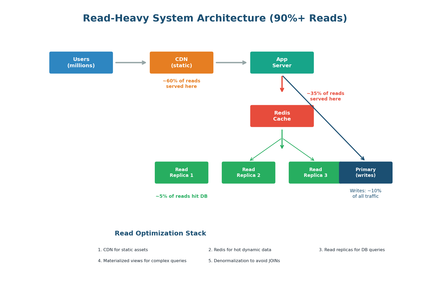
Read-Heavy Systems: Cache Everything
In a read-heavy system (>80% reads), the primary goal is to serve reads as fast as possible while minimizing database load. The architecture follows a layered caching approach: CDN caches static assets and cacheable API responses at the edge (~60% of reads). Redis caches dynamic data in memory (~35% of reads). Read replicas handle the remaining ~5% of reads that miss all caches. The primary database handles only writes and the occasional cache-miss read.
1. Aggressive Caching (Redis + CDN): Cache everything that does not change every second. User profiles, product pages, feed items, configuration — all belong in Redis. Set appropriate TTLs: 5 seconds for real-time data, 60 seconds for user data, 24 hours for product catalogs. A 95% cache hit rate means only 5% of reads touch the database.
2. Read Replicas: Add 2–5 read replicas for the 5% of reads that miss cache. Route read queries to replicas, reserving the primary for writes. With 3 replicas, you have 4x total read capacity compared to a single server.
3. Denormalization: Pre-compute JOINs and store the result. Instead of joining users + orders + products at query time, store a denormalized user_feed table with everything pre-joined. This trades write complexity for read speed — a deliberate choice in read-heavy systems.
4. Materialized Views: Pre-computed query results stored as a table. When the underlying data changes, the view is refreshed (async or periodically). Perfect for dashboards and analytics that need complex aggregations but tolerate slightly stale data.
Write-Heavy Systems: Buffer and Distribute
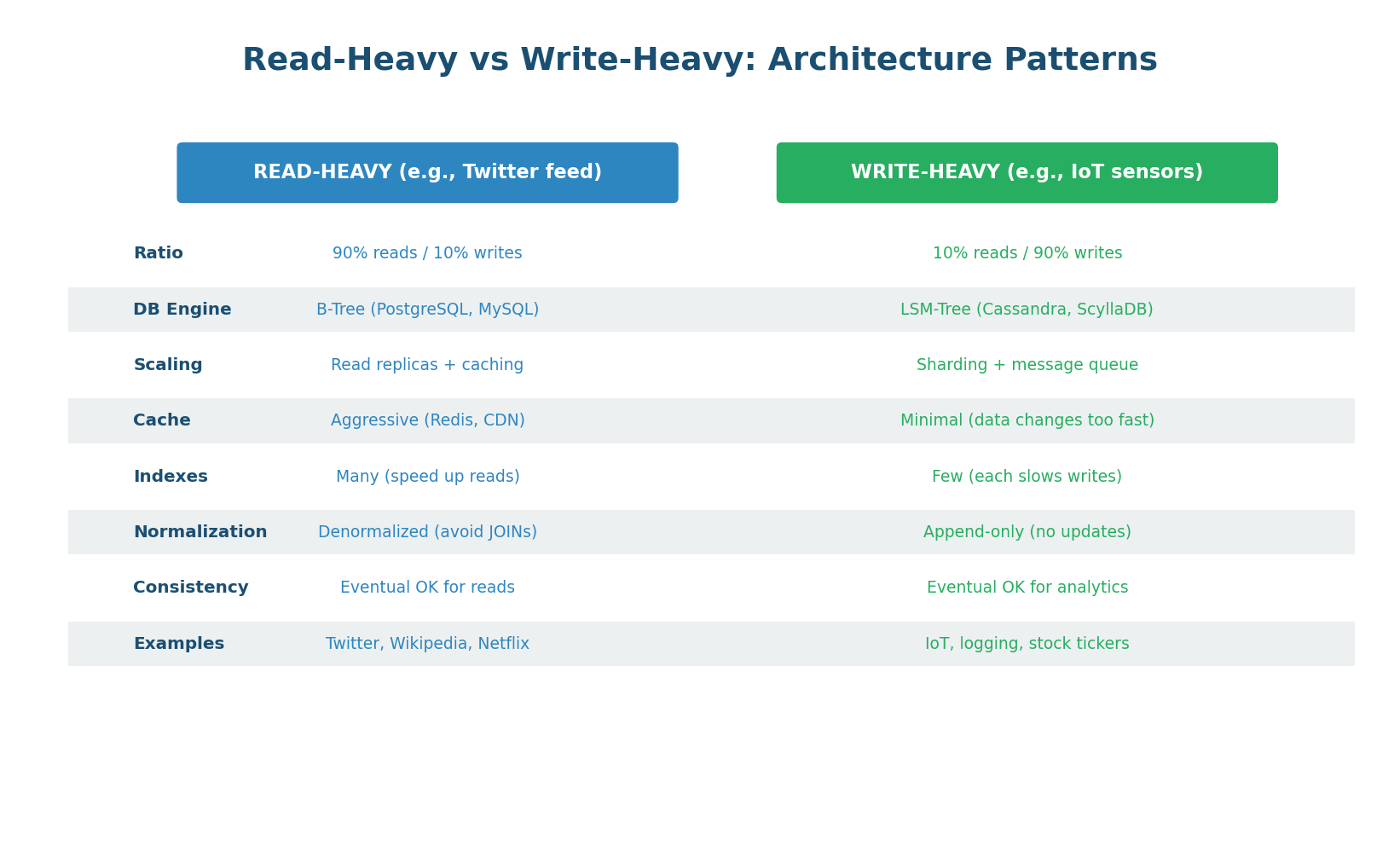
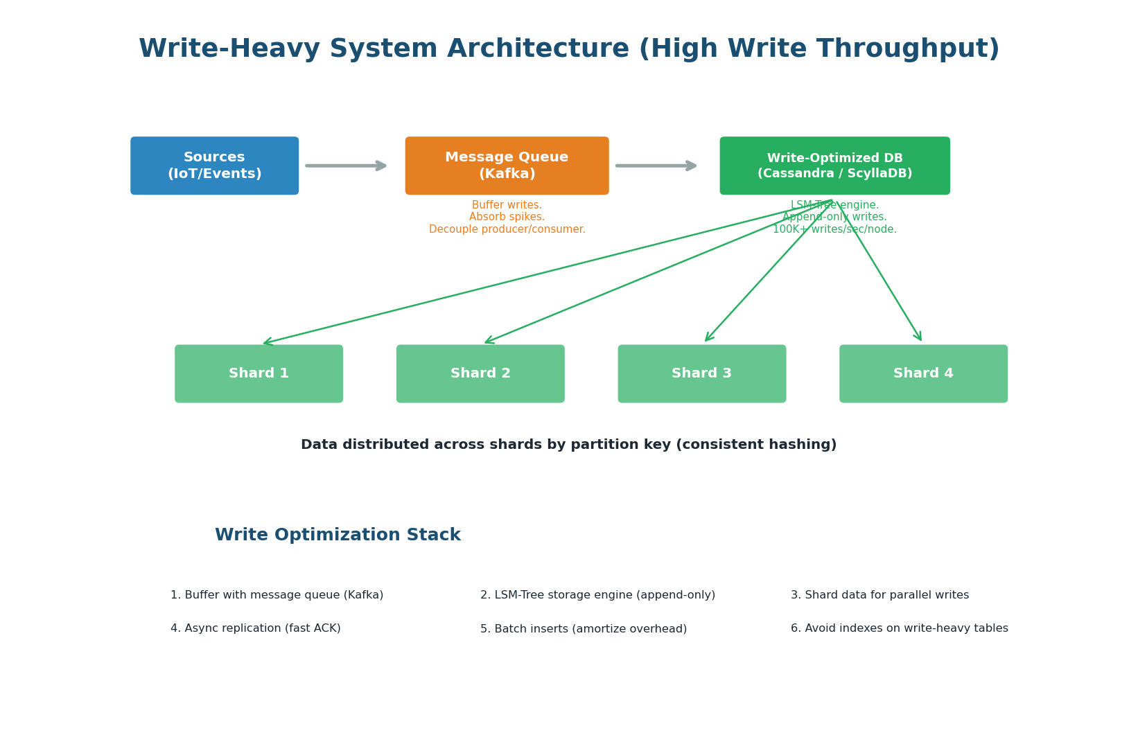
In a write-heavy system (>80% writes), the primary goal is to absorb writes at massive scale without data loss. The architecture uses a write-ahead buffer (Kafka), a write-optimized storage engine (LSM-Tree based like Cassandra), and sharding to parallelize writes across multiple machines.
1. Message Queue Buffer (Kafka): Never write directly to the database from the application. Instead, publish write events to Kafka, which buffers them durably. A separate consumer processes events and writes to the database at a controlled rate. This absorbs traffic spikes: even if 1 million events arrive in 1 second, Kafka buffers them, and the consumer writes at a sustainable 100K/sec.
2. LSM-Tree Storage Engine: Choose Cassandra, ScyllaDB, or another LSM-Tree based database. Sequential writes (append-only) are 5–10x faster than random I/O (B-Tree update-in-place). A single Cassandra node can handle 50–100K writes/sec.
3. Sharding for Parallel Writes: Distribute data across multiple shards so writes are parallelized. 4 shards = 4x write throughput. Use consistent hashing on the partition key for even distribution.
4. Minimize Indexes: Every index on a write-heavy table is a write amplifier. If a table has 5 indexes, each INSERT triggers 6 write operations (1 row + 5 index updates). Keep only essential indexes. Consider writing raw data and indexing asynchronously in a separate read store.
5. Batch Writes: Instead of 1,000 individual INSERTs, batch them into a single INSERT with 1,000 rows. This amortizes network round-trip, transaction overhead, and disk flush costs. Cassandra's BATCH statement and PostgreSQL's COPY command support this natively.
Discord stores trillions of messages across billions of conversations. Their access pattern is write-heavy (millions of messages sent per minute) but also requires fast reads. They use Cassandra with a partition key of (channel_id, bucket) where bucket groups messages by time window. Writes are always appends (LSM-Tree, fast). Reads fetch the last N messages in a channel (single partition, fast). This single architecture decision — choosing Cassandra's LSM-Tree over PostgreSQL's B-Tree — is what makes Discord's message storage work at scale.
CQRS: When You Need Both
Some systems are both read-heavy AND write-heavy — they need high write throughput and fast, complex reads. The solution is CQRS (Command Query Responsibility Segregation): use a separate optimized database for writes and a separate optimized database for reads, synchronized via an event stream.
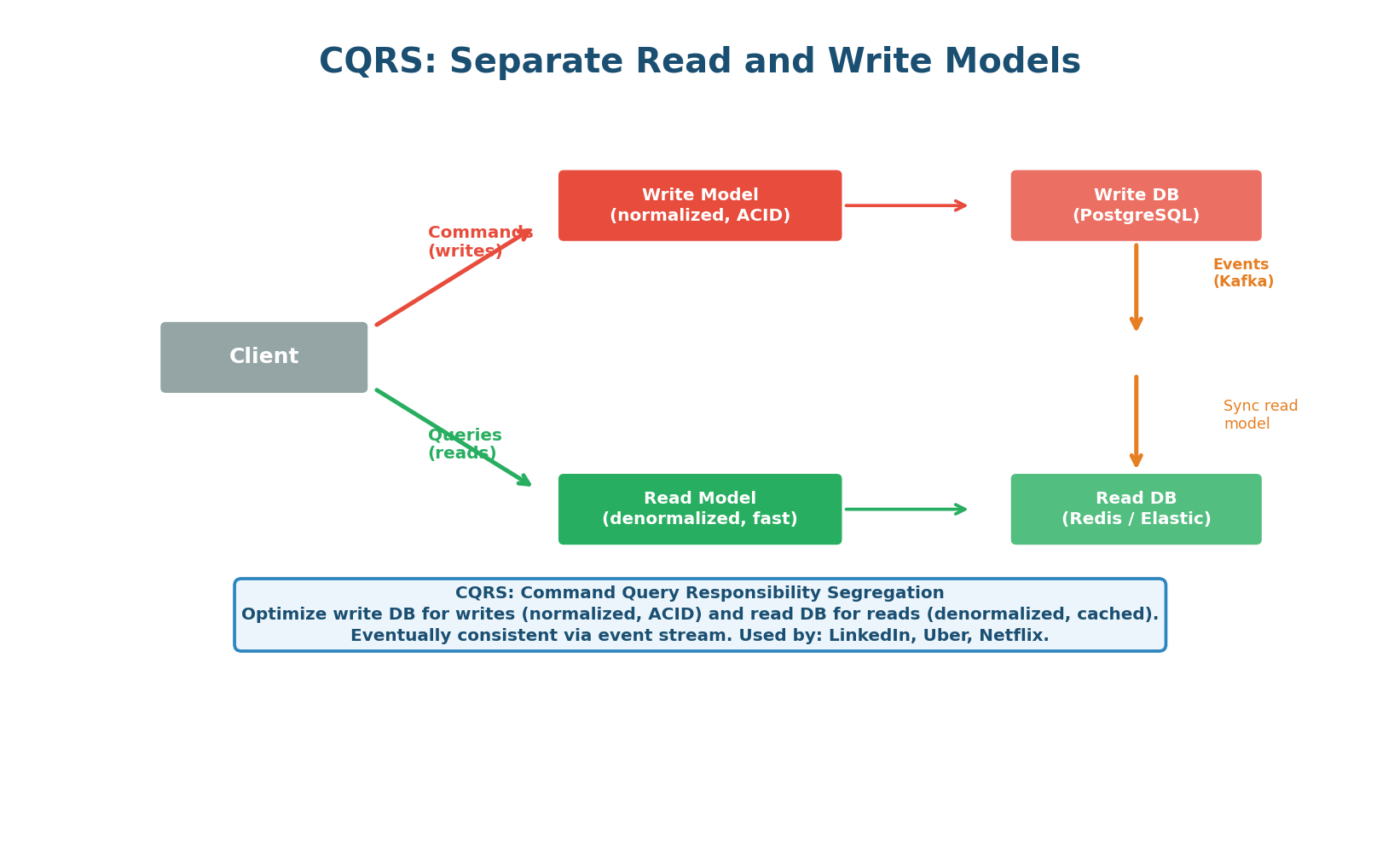
In CQRS, the write model uses a normalized relational database (PostgreSQL) for ACID transactions. When data changes, events are published to Kafka. The read model consumes these events and updates a denormalized read store (Redis, Elasticsearch, or a materialized view) optimized for the specific read queries your application needs. The read store is eventually consistent with the write store (typically 10–100ms behind).
| Aspect | Traditional (Single DB) | CQRS |
|---|---|---|
| Write store | General-purpose DB | ACID-optimized DB (PostgreSQL) |
| Read store | Same DB (read replicas) | Query-optimized store (Redis, Elasticsearch) |
| Consistency | Strong (reads always current) | Eventual (read store lags by 10–100ms) |
| Read performance | Limited by write schema | Unlimited — read store tailored to query |
| Complexity | Low | High (sync pipeline, eventual consistency) |
| When to use | Most systems (<100K QPS) | High-scale systems needing both fast writes and complex reads |
CQRS adds enormous complexity: you must manage two databases, a synchronization pipeline, and eventual consistency in your application code. Only use CQRS when you have a proven need that cannot be met by a simpler architecture. Start with a single PostgreSQL database with read replicas and Redis caching. Graduate to CQRS only when you can measure the specific bottleneck it solves.
Topic 3
Partitioning Strategies
Horizontal vs Vertical Partitioning
Partitioning splits a large dataset into smaller, more manageable pieces. There are two fundamentally different approaches: horizontal partitioning (sharding) splits rows across multiple databases, and vertical partitioning splits columns into separate tables. Both reduce the amount of data any single query needs to process, but they solve different problems.
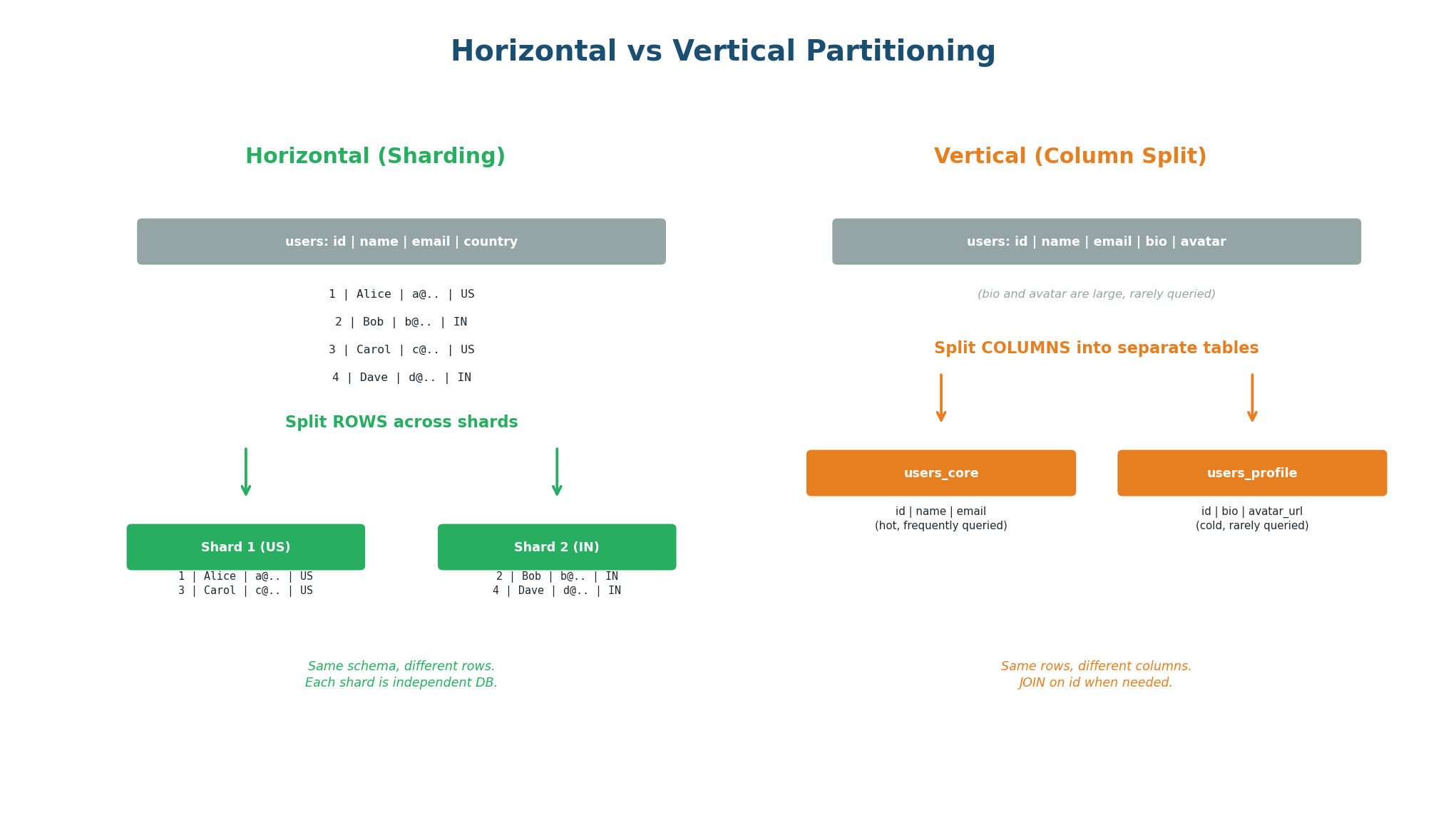
Horizontal Partitioning (Sharding): Each shard contains a subset of rows with the full schema. Shard 1 might hold users with IDs 1–100K, Shard 2 holds 100K–200K, and so on. Each shard is an independent database that handles both reads and writes for its subset. This scales both read and write throughput linearly: 4 shards = 4x capacity. The challenge is choosing the right partition key and handling cross-shard queries.
Vertical Partitioning (Column Splitting): Splits a wide table into multiple narrower tables. A users table with 50 columns might be split into users_core (id, name, email — queried frequently) and users_profile (id, bio, avatar, preferences — queried rarely). This reduces the data read per query (smaller rows = more rows per page = faster scans) and allows different storage tiers (hot columns on SSD, cold columns on HDD). Vertical partitioning is often overlooked but is far simpler than sharding.
| Aspect | Horizontal (Sharding) | Vertical (Column Splitting) |
|---|---|---|
| What it splits | Rows across multiple databases | Columns into separate tables |
| What it solves | Data volume + write throughput | Wide tables, I/O efficiency, access frequency |
| Complexity | Very high (cross-shard queries, rebalancing) | Low (just a schema change) |
| When to use | Data exceeds one machine or write throughput limit | Tables with many columns, mixed access patterns |
| Try first? | No — last resort | Yes — always consider this first |
Partition Key Selection: The Most Critical Decision
The partition key determines which shard holds each piece of data. A good partition key has high cardinality (millions of unique values), produces even distribution across shards, and matches your primary query pattern (most queries include the partition key in the WHERE clause).
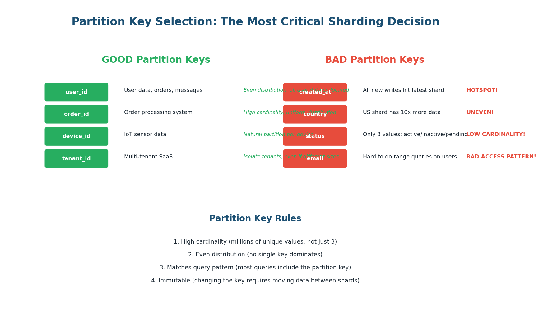
| Partition Key | Cardinality | Distribution | Verdict |
|---|---|---|---|
user_id (UUID) | Very high (billions) | Even (random UUIDs) | Excellent |
user_id (auto-increment) | High | Even (with hash) | Good |
country | Low (~200) | Very uneven (US > others) | Poor — hotspot risk |
status (active/inactive) | Very low (2) | Extremely uneven | Never use alone |
created_at (date) | High | Uneven (latest date gets all writes) | Poor for writes |
(user_id, created_at) | Very high | Even + time-ordered per user | Excellent for messaging |
The Hot Partition Problem (Celebrity Problem)
Even with a good partition key, some partitions can become disproportionately hot. If you shard by user_id and one user has 100 million followers (Justin Bieber), the shard containing that user receives 100x more read traffic than average shards. This is the celebrity problem, and it can bring down an entire shard while others sit idle.
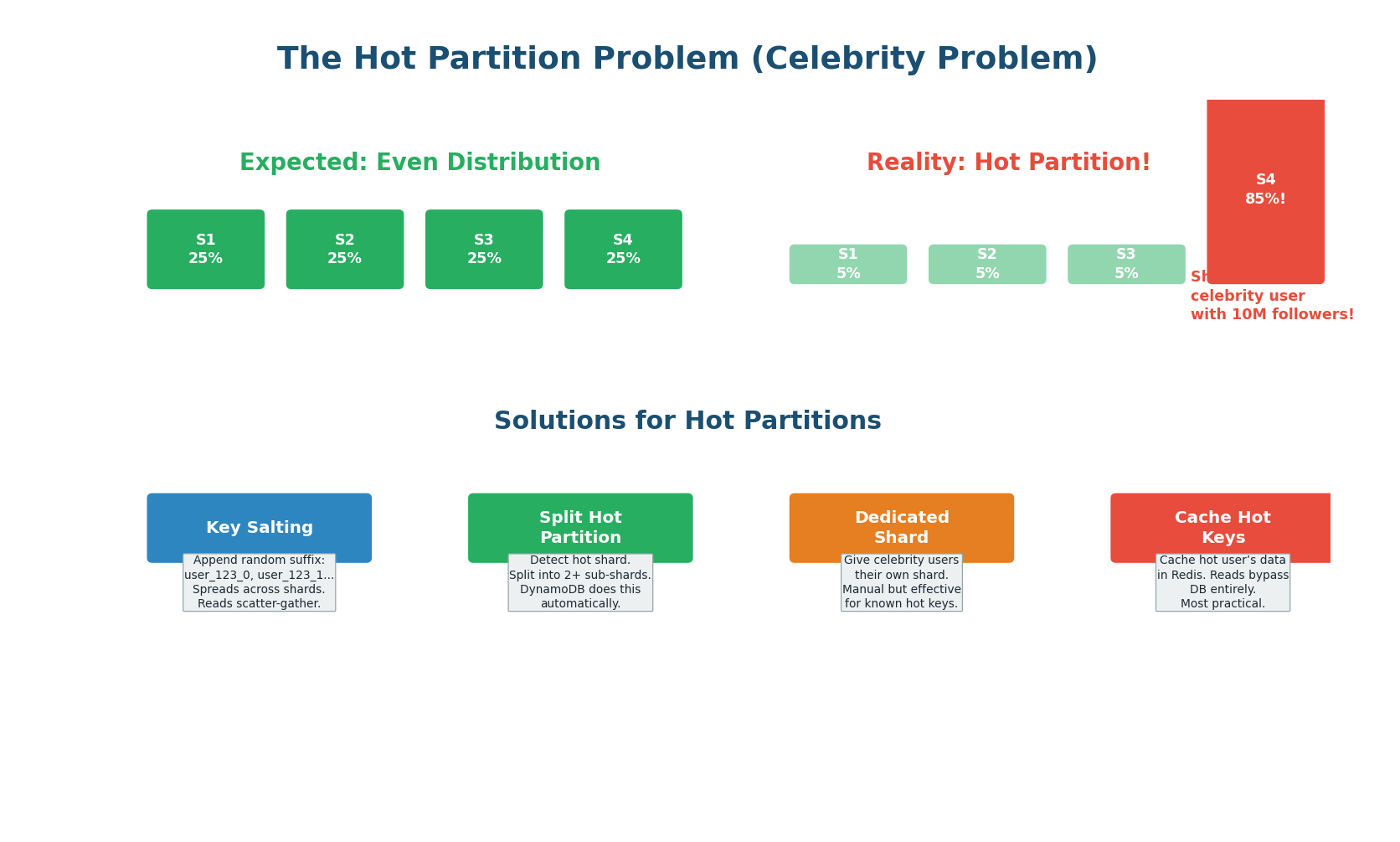
Solution 1: Cache Hot Keys (Most Practical). Identify the top N hot keys via monitoring and cache their data in Redis. All reads for hot keys are served from cache, bypassing the database entirely. The hot shard's load drops dramatically because 99% of its traffic was reads for the celebrity user, and those reads now hit Redis instead. This is the most practical solution for most systems.
Solution 2: Key Salting. Append a random suffix (0–9) to the hot key: user_123_0, user_123_1, ..., user_123_9. These 10 keys hash to different shards, spreading the load across 10 partitions instead of 1. The trade-off: reads for user 123 must now scatter-gather across all 10 partitions and merge the results. This adds read latency but prevents write hotspots. Best for write hotspots.
Solution 3: Dynamic Shard Splitting. Monitor shard utilization and automatically split hot shards into smaller sub-shards. DynamoDB does this automatically: when a partition exceeds its throughput limit, DynamoDB transparently splits it. The application does not need to change. This is the most operationally simple solution if your database supports it.
Solution 4: Dedicated Shard for Hot Keys. Identify known hot keys in advance (top celebrities, viral products) and route them to a dedicated, higher-capacity shard. This shard gets beefier hardware or more replicas. Combined with caching, this handles even the most extreme hotspots.
Database Selection Guide
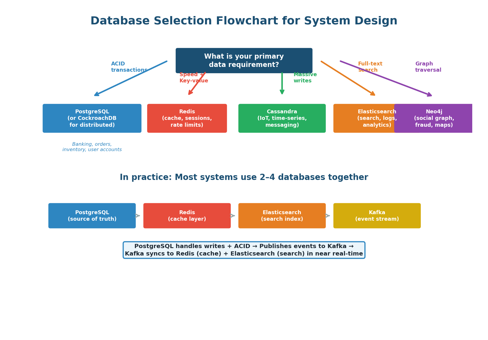
In practice, no single database handles all requirements. A typical production system uses multiple databases, each chosen for a specific job:
| Database | Primary Role | Why |
|---|---|---|
| PostgreSQL | Source of truth, transactional data | ACID, complex queries, strong consistency |
| Redis | Caching, sessions, real-time counters | Sub-millisecond reads, data structures |
| Cassandra / ScyllaDB | Write-heavy append workloads | LSM-Tree, 100K+ writes/sec per node |
| Elasticsearch | Full-text search, log analytics | Inverted index, fast text queries |
| Kafka | Event streaming, write buffering | Durable, high-throughput, decouples producers from consumers |
| S3 / Object Storage | Binary blobs (images, videos, docs) | Cheap, infinitely scalable, CDN-compatible |
When asked "what database would you use?", never name just one. Show your depth: "I would use PostgreSQL as the source of truth for user accounts and orders — ACID guarantees are non-negotiable here. Redis for session tokens and rate limiting (sub-millisecond latency). Elasticsearch for full-text product search. Kafka as the event bus between these systems so they stay in sync. Object storage (S3) for product images. Each database is chosen because it is the best tool for that specific job."
Class Summary
Connecting the Three Topics
Database Trade-offs are rooted in the storage engine choice. B-Trees (PostgreSQL, MySQL) optimize for reads with predictable O(log N) performance. LSM-Trees (Cassandra, RocksDB) optimize for writes with 5–10x throughput via sequential I/O. The trade-off triangle (reads vs writes vs storage) governs every architectural decision — every optimization costs something else.
Read-Heavy vs Write-Heavy systems require fundamentally different architectures. Read-heavy systems use aggressive caching (CDN + Redis), read replicas, and denormalization to ensure 95% of reads never touch the database. Write-heavy systems use message queues (Kafka), LSM-Tree databases (Cassandra), sharding, and minimal indexes. CQRS lets you optimize both independently when you need both — but at significant complexity cost.
Partitioning Strategies determine how data is distributed across machines. Vertical partitioning (column splitting) is simple and should always be tried first. Horizontal partitioning (sharding) scales both reads and writes but adds enormous complexity. The partition key must have high cardinality, even distribution, and match your query pattern. Hot partitions are solved by caching hot keys first, then key salting, dynamic splitting, or dedicated shards as needed.
Want to Land at Google, Microsoft or Apple?
Watch Pranjal Jain's free 30-min training — the exact GROW Strategy that helped 1,572+ engineers go from TCS/Infosys to top product companies with a 3–5X salary hike.