
What's Inside
Topic 1
Latency vs Throughput vs Bandwidth
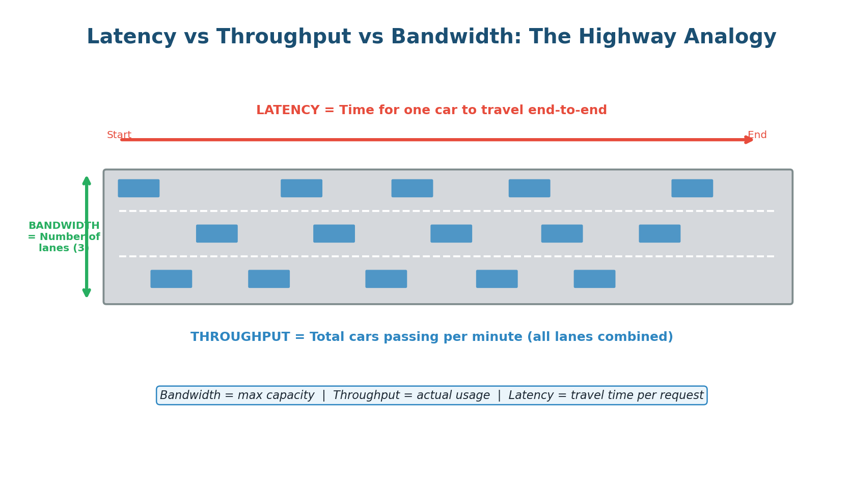
Every system designer must understand three fundamental performance metrics: Latency, Throughput, and Bandwidth. These three concepts describe different dimensions of system performance, and confusing them is a common mistake in interviews. They are related but distinct — like speed, traffic volume, and road width on a highway.
Latency: How Fast Is a Single Request?
Latency is the time it takes for a single request to travel from the sender to the receiver and back (round-trip), or for an operation to complete. It is measured in milliseconds (ms) or microseconds (µs). When you click a link and the page takes 200ms to load, that 200ms is the latency.
Latency is what users feel directly. A system with 50ms latency feels instant. A system with 500ms latency feels sluggish. A system with 2,000ms latency feels broken. Google found that adding just 500ms of latency to search results reduced traffic by 20%. Amazon found that every 100ms of added latency cost them 1% in sales. Latency is money.
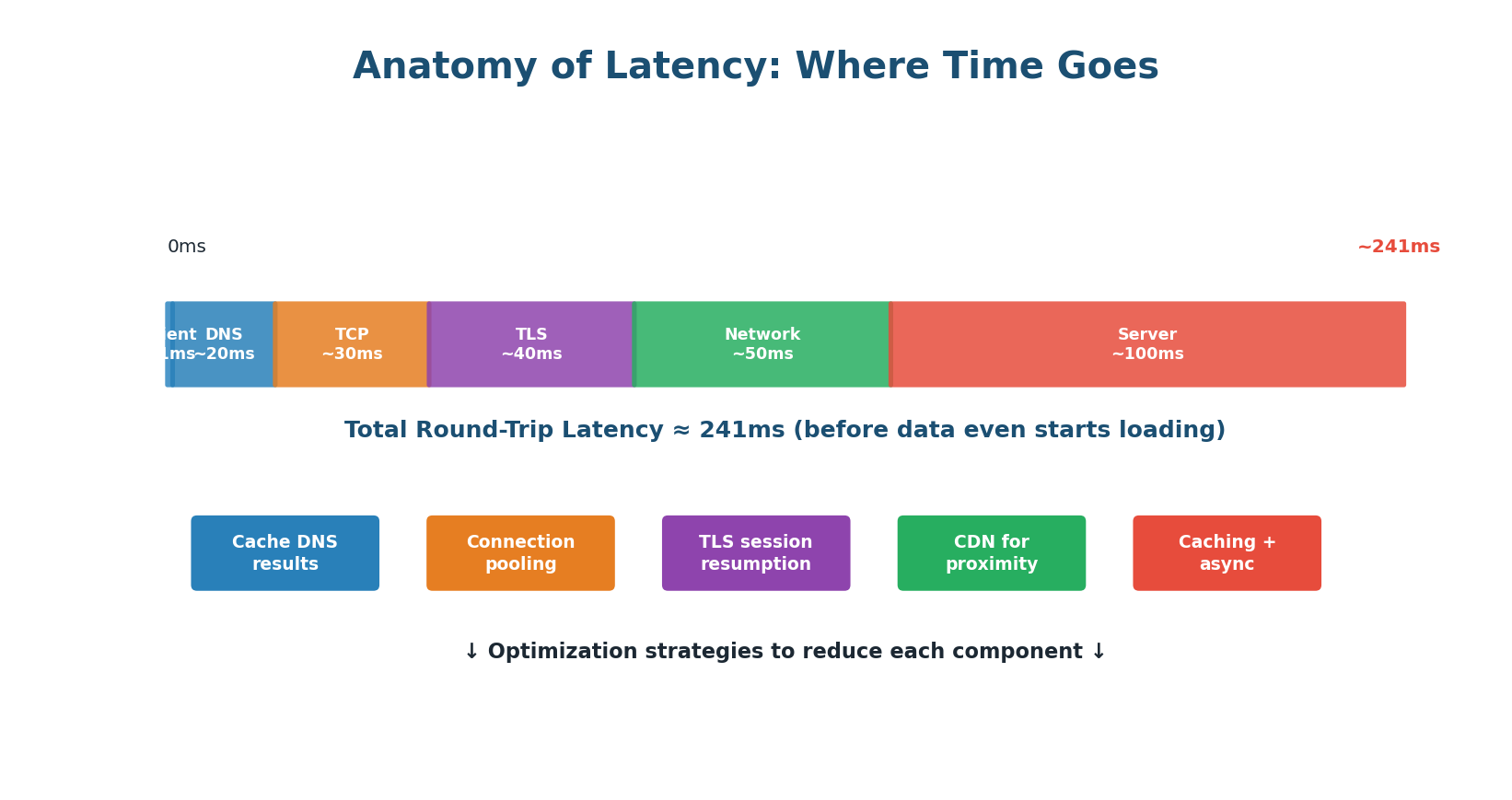
A single request passes through many stages, each adding latency:
- Client Processing (~1ms): The browser or app prepares the request. Usually negligible.
- DNS Lookup (~20ms): Domain name resolved to IP address. Can take 20–100ms for first request; cached after.
- TCP Handshake (~30ms): Three-way handshake (SYN, SYN-ACK, ACK) requires one full round-trip.
- TLS/SSL Handshake (~40ms): For HTTPS connections, an additional 1–2 round-trips to exchange certificates.
- Network Transfer (~50ms): Depends on physical distance, number of hops, and congestion.
- Server Processing (~100ms): Database queries, computation, business logic. The largest and most controllable component.
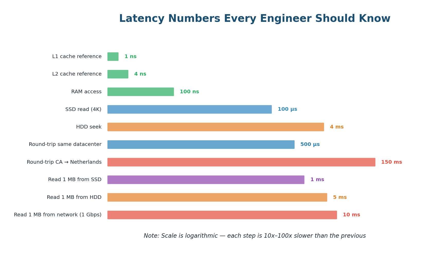
Latency Numbers Every Engineer Should Know
| Operation | Approximate Latency | Relative Speed |
|---|---|---|
| L1 cache reference | ~0.5 ns | Baseline |
| L2 cache reference | ~7 ns | 14× slower |
| RAM read | ~100 ns | 200× slower |
| SSD random read | ~100 µs | 200,000× slower |
| HDD seek | ~10 ms | 20,000,000× slower |
| Round-trip in same DC | ~0.5 ms | 1,000,000× slower |
| Cross-continent round-trip | ~150 ms | 300,000,000× slower |
Reading from RAM is ~100,000× faster than reading from SSD. A network round-trip across the Atlantic takes 150 million times longer than reading from L1 cache. This is why caching is so impactful — moving a database query result from disk to memory can be a 100,000× improvement.
Throughput and Bandwidth
Throughput is the total amount of work a system can handle per unit of time — measured in requests per second (RPS), transactions per second (TPS), or data transferred per second (MB/s). While latency measures the speed of a single request, throughput measures the total volume of requests the system can process simultaneously.
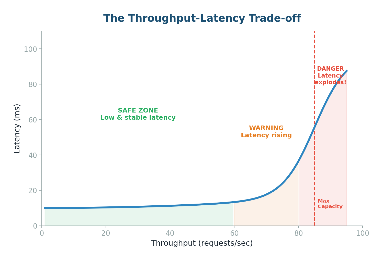
As you push throughput higher, latency stays stable for a while, then suddenly explodes:
- Safe Zone (below ~60% capacity): System has headroom. Requests processed immediately with consistent, low latency.
- Warning Zone (60–80% capacity): Queues start to form. Average latency rises; p99 latency rises faster.
- Danger Zone (above 80%): System is saturated. Queues grow exponentially. Latency spikes to seconds. System may crash.
Bandwidth is the theoretical maximum data transfer capacity — the number of highway lanes. Throughput is the actual usage. Key relationship: Throughput ≤ Bandwidth. As throughput approaches bandwidth, latency increases exponentially due to congestion.
| Metric | Definition | Analogy | Measured In |
|---|---|---|---|
| Latency | Time for one request to complete | Travel time per car | ms, µs |
| Throughput | Work done per unit time | Cars per minute on highway | RPS, TPS, MB/s |
| Bandwidth | Maximum data transfer capacity | Number of highway lanes | Mbps, Gbps |
Topic 2
Consistent Hashing
The Problem: Why Simple Hashing Breaks
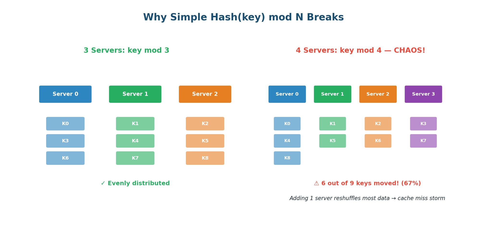
Imagine you have 3 database servers and 9 data keys. The simplest way to distribute data is: server = Hash(key) mod N, where N is the number of servers. This distributes data evenly and is easy to implement.
But now you add a 4th server. N changes from 3 to 4. Suddenly, 6 out of 9 keys are now assigned to different servers. If these keys were cached in memory, you just invalidated 67% of your cache. Every one of those 6 keys triggers a cache miss, hitting the database directly. With millions of keys, this causes a "cache miss storm" that can overwhelm your database and cause a cascading failure.
The Hash Ring
Consistent hashing, popularized by Amazon's Dynamo paper, solves this problem elegantly. Instead of mapping keys to servers using modular arithmetic, both keys and servers are placed on a circular ring (the hash ring). When you add or remove a server, only approximately K/N keys need to move — where K is the total number of keys and N is the number of servers.
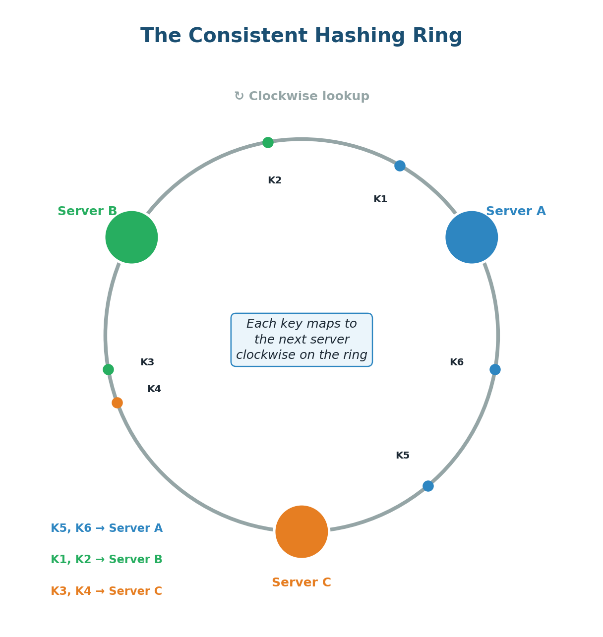
The core idea:
- Create a circular hash space (ring) from 0 to some maximum value (e.g., 0 to 2³² - 1).
- Hash each server's identifier (IP address or name) to a position on the ring.
- Hash each data key to a position on the same ring.
- To find which server owns a key: start at the key's position and walk clockwise around the ring until you reach a server. That server owns the key.
Adding a server: When you add Server D, it takes a position between two existing servers. Only the keys in the range between D's position and the previous server (counter-clockwise) need to move to D. All other keys stay where they are — roughly 1/N of keys move instead of N-1/N.
Removing a server: When Server B fails, only B's keys move. They are reassigned to the next server clockwise. All keys assigned to other servers remain untouched. The impact is localized.
Virtual Nodes: Solving Uneven Distribution
Basic consistent hashing has a problem: with only a few servers, the positions on the ring can be uneven. Servers might cluster together, causing one server to own a huge chunk of the ring (and thus a disproportionate number of keys).
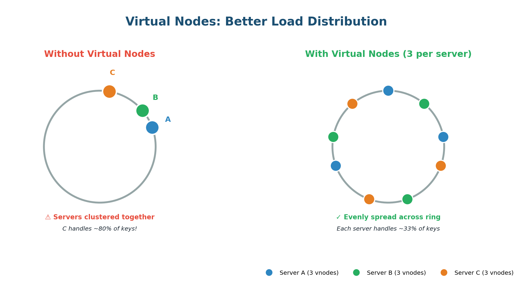
Virtual nodes (VNodes) solve this by giving each physical server multiple positions on the ring. Instead of hashing each server once, you hash it multiple times (Server-A-0, Server-A-1, Server-A-2, etc.). In practice, systems like Cassandra use 256 virtual nodes per physical server by default.
Virtual nodes elegantly handle servers with different capacities. If Server A has 2× the memory and CPU of Server B, simply assign Server A twice as many virtual nodes. Server A gets 200 positions while Server B gets 100. Server A naturally receives roughly twice as many keys, matching its capacity.
Apache Cassandra, Amazon DynamoDB, Discord message routing, Akamai CDN, Redis Cluster, Riak, and Chord DHT. Any system where data must be distributed across many nodes and nodes are added/removed dynamically.
Topic 3
The CAP Theorem
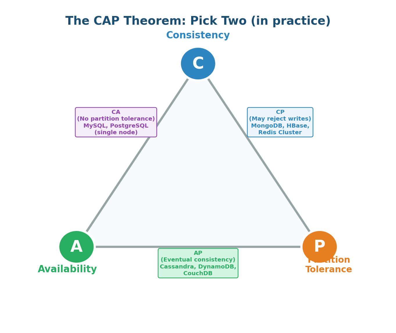
The CAP Theorem, proposed by Eric Brewer in 2000, states that a distributed data store can only guarantee two out of three properties simultaneously: Consistency (C), Availability (A), and Partition Tolerance (P). In the presence of a network partition, you must choose between Consistency and Availability.
| Property | Definition | What It Means in Practice |
|---|---|---|
| Consistency (C) | Every read receives the most recent write or an error | All nodes see the same data at the same time (linearizability) |
| Availability (A) | Every request receives a non-error response | System always responds, even if the data may be slightly stale |
| Partition Tolerance (P) | System continues to operate despite network partitions | Network failures between nodes don't bring the system down |
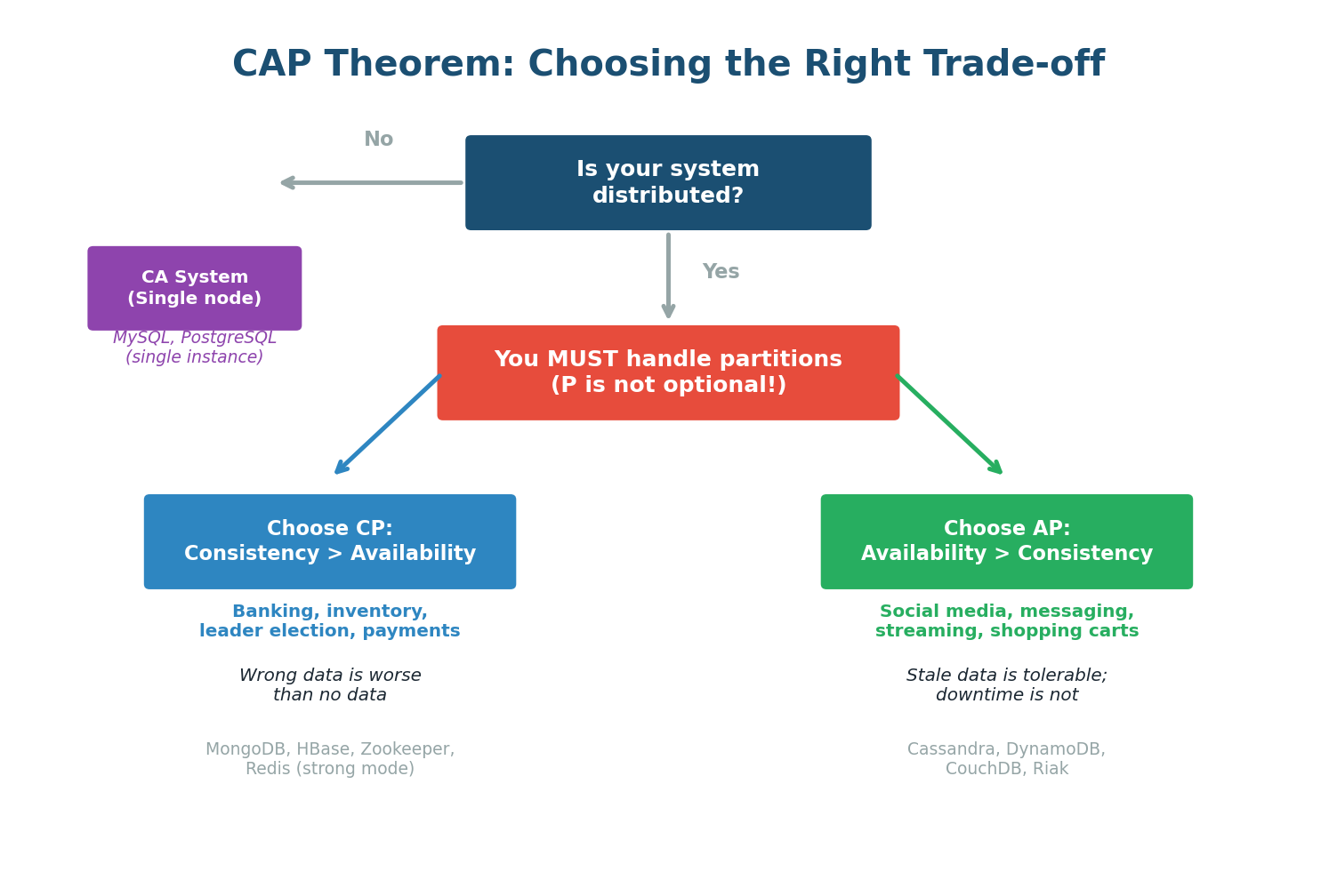
In any distributed system deployed across multiple machines, network partitions are inevitable — they happen due to cable cuts, router failures, data center issues, or software bugs. This is why the practical version of CAP is: since P is mandatory, you must choose between C and A during a partition.
CP vs AP: The Real Choice
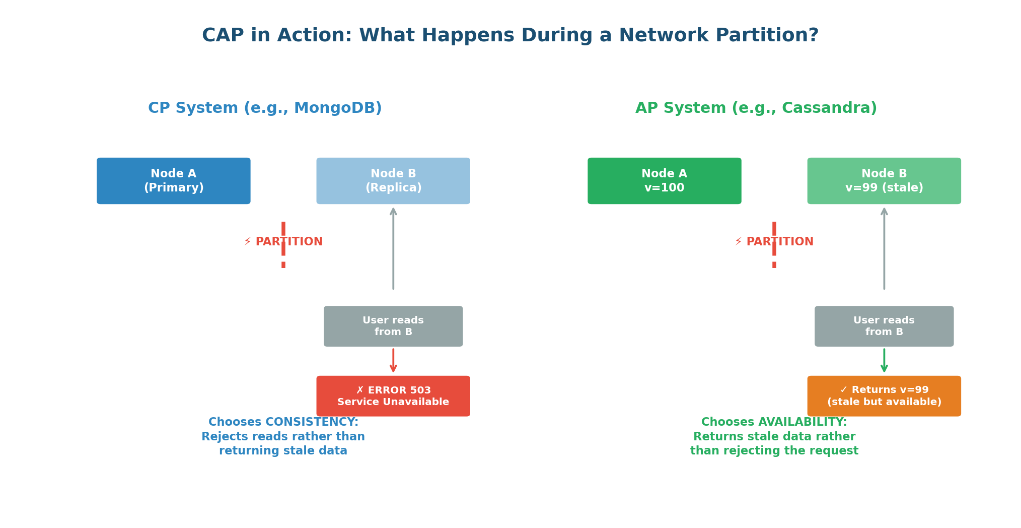
CP Systems: When a network partition occurs, CP systems refuse to serve potentially stale data. They return an error rather than risking an inconsistent response. Users might see "Service Unavailable," but they will never see incorrect data.
Banking and financial systems (wrong balances lose money), inventory systems (overselling is expensive), leader election and coordination services (split-brain is dangerous), any system where incorrect data is worse than no data. Examples: MongoDB, HBase, Zookeeper, etcd, Redis Cluster.
AP Systems: When a network partition occurs, AP systems continue serving requests from all nodes, even if some nodes have stale data. Every request gets a response, but the data might be slightly outdated. After the partition heals, the system reconciles conflicting data.
Social media (stale posts are acceptable), messaging (eventual delivery is fine), shopping carts (merge on reconciliation), DNS (slightly stale records are acceptable). Examples: Cassandra, DynamoDB, CouchDB, Riak.
Beyond CAP: PACELC & Tunable Consistency
CAP is per-operation, not per-system. Your banking system might be CP for balance updates but AP for transaction history queries. Cassandra lets you configure consistency per query: QUORUM reads give strong consistency, ONE reads give availability.
PACELC extends CAP by asking: even when there is no partition, what trade-off do you make? PACELC says: if there is a Partition, choose between A or C; Else (no partition), choose between Latency and Consistency. DynamoDB defaults to eventually consistent reads (faster) but offers strongly consistent reads (slower) as an option.
| Write Quorum (W) | Read Quorum (R) | W+R > N? | Result |
|---|---|---|---|
| ALL (3) | ONE (1) | 4 > 3 ✓ | Strong consistency, slow writes |
| QUORUM (2) | QUORUM (2) | 4 > 3 ✓ | Strong consistency, good availability |
| ONE (1) | ONE (1) | 2 < 3 ✗ | Eventual consistency, max speed |
Class Summary
Connecting the Dots
Today's three topics are deeply interconnected and form the technical backbone of every distributed system design:
- Latency, Throughput, and Bandwidth give you the vocabulary to quantify system performance. When you say "I need sub-100ms latency at 1.2M QPS," you are setting concrete targets that drive architectural decisions.
- Consistent Hashing gives you the mechanism to distribute data across multiple servers as you scale horizontally. Without it, every scaling event causes massive data redistribution and cache invalidation.
- The CAP Theorem gives you the framework to make fundamental decisions about data consistency and availability. Once you distribute data using consistent hashing across multiple nodes, you must face the CAP trade-off.
Together, these three concepts let you design a system that is fast (low latency, high throughput), scalable (consistent hashing for data distribution), and resilient (CAP-aware trade-offs for distributed data).
Want to Land at Google, Microsoft or Apple?
Watch Pranjal Jain's free 30-min training — the exact GROW Strategy that helped 1,572+ engineers go from TCS/Infosys to top product companies with a 3–5X salary hike.