
What's Inside
Topic 1
Partitioning Trade-offs
What You Gain vs What You Lose
Partitioning (sharding) is the most powerful and most costly scaling technique in your toolbox. It allows you to exceed the capacity of a single machine by distributing data across multiple machines. The decision to shard is irreversible in most architectures — you cannot easily un-shard later — so understanding the trade-offs before committing is critical.
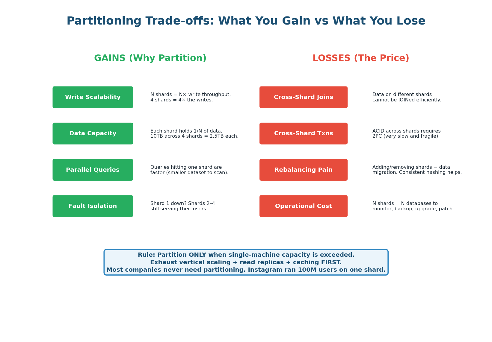
The Gains:
- Write Scalability: A single PostgreSQL node maxes out at ~50K writes/second. With 4 shards, you get 200K writes/second because each shard handles its own subset. This is the primary reason to shard — writes cannot be parallelized within a single node.
- Data Capacity: A single node's disk is finite (typically 1–16 TB). With 4 shards, you store 4x the data. Google Spanner uses thousands of shards to store petabytes. Each shard is a manageable chunk of data with its own index.
- Parallel Queries: A full-table scan that takes 10 minutes on one node takes 2.5 minutes across 4 shards in parallel (scatter-gather). Analytical workloads benefit enormously from this.
- Fault Isolation: If Shard 1 goes down, Shards 2–4 still serve their users. A single-node database is a single point of failure for all data.
The Losses:
- Cross-Shard Joins: If User 42's orders are on Shard 1 and Product 99's details are on Shard 3, a JOIN requires querying both shards, transferring data over the network, and merging results in application code. This scatter-gather pattern has high latency and operational complexity.
- Cross-Shard Transactions: ACID transactions across shards require two-phase commit (2PC), which is slow (2x latency), fragile (coordinator crash = blocked transactions), and reduces availability. The practical advice: design your data model to avoid cross-shard transactions.
- Rebalancing Pain: When you add a new shard, data must be migrated from existing shards. This is an expensive, disruptive operation. Consistent hashing minimizes the data movement but doesn't eliminate it.
- Operational Complexity: Each shard is an independent database server: backups, monitoring, schema migrations, and failover must be managed N times. Your ops burden scales with shard count.
In interviews, propose sharding only when you've exhausted vertical scaling and read replicas. Start with a single large node, add read replicas, then shard when writes become the bottleneck. The interviewer will ask: "How did you decide to shard?" The answer is: when write throughput exceeded what a single primary can handle.
Partition Key Trade-off: Locality vs Distribution
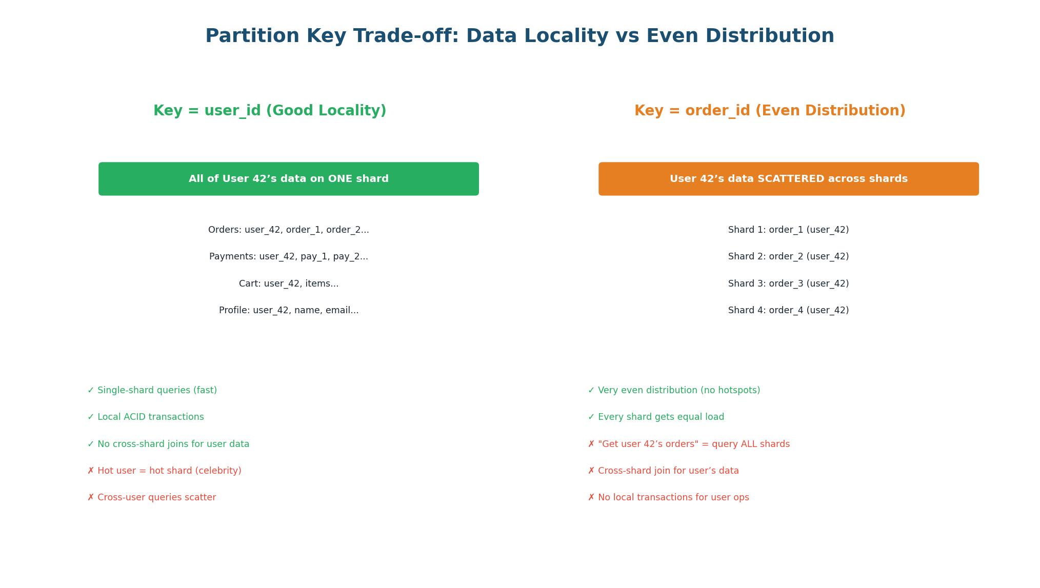
The partition key determines two things: how evenly data is distributed (avoiding hotspots) and how much data is co-located (enabling local queries). These two goals are in direct tension — you cannot fully optimize for both at once.
| Partition Key | Locality | Distribution | Hotspot Risk | Best For |
|---|---|---|---|---|
user_id | All user data on one shard | Skewed if power users exist | High (celebrity problem) | Social apps with user-centric queries |
order_id | Order data scattered | Even (random IDs) | Low | Order processing, analytics |
geography | Regional data co-located | Skewed by population | Medium (dense regions) | Geo-local apps (food delivery) |
hash(user_id) | None (hash destroys locality) | Even | Very low | Pure write throughput, no range queries |
Twitter's original sharding used user_id. When a celebrity with 100M followers tweeted, one shard received 100x the normal write load as fanout jobs wrote to follower timelines. The fix: special-case celebrity accounts (users with >1M followers) and precompute their fan-out differently, bypassing the shard bottleneck.
Topic 2
Replication Strategies
Three Replication Topologies
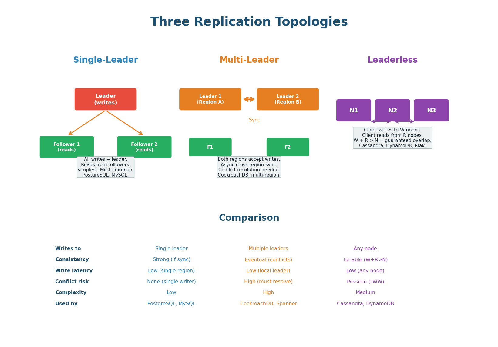
Replication copies data across multiple nodes for three reasons: durability (data survives node failures), read scaling (distribute reads across replicas), and geographic proximity (replicas near users reduce latency). The topology determines how writes flow through the system.
| Topology | Write Path | Consistency | Conflict Risk | Real Systems |
|---|---|---|---|---|
| Single-Leader | All writes → one primary → replicated to followers | Strong (sync replication) or eventual (async) | None (one writer) | PostgreSQL, MySQL, MongoDB, Redis Sentinel, Kafka (per partition) |
| Multi-Leader | Each region has a leader, leaders replicate to each other | Eventual (async cross-region) | High (concurrent writes to same key in different regions) | CockroachDB, Google Spanner, DynamoDB Global Tables |
| Leaderless | Client writes to W nodes simultaneously, reads from R nodes | Tunable (W+R > N = strong) | Medium (concurrent writes to same key) | Cassandra, DynamoDB, Riak |
Single-Leader (Primary-Replica): One node (the leader/primary) accepts all writes. It replicates changes to followers (replicas) via a replication log. Followers are read-only. This is the simplest and most common topology. Consistency is configurable: synchronous replication (follower must ACK before primary responds — strong consistency, lower throughput) or asynchronous (primary responds immediately, replicates in background — eventual consistency, higher throughput). Use this as your default in any interview where strong consistency matters.
Multi-Leader (Active-Active): Multiple nodes in different regions each accept writes. Changes are replicated asynchronously between leaders. This gives low write latency for users in each region (writes go to the local leader). The challenge: if two users in different regions update the same record simultaneously, you have a write conflict. Use only when you need low-latency writes across multiple geographic regions and you have a conflict resolution strategy.
Leaderless (Dynamo-style): No designated leader. The client writes to W nodes and reads from R nodes. If W + R > N (total replicas), reads and writes overlap, guaranteeing the client reads the latest write. The most flexible topology but requires the application to handle stale reads and version conflicts. Choose when you need high availability and can tolerate eventual consistency.
Quorum Reads & Writes: Tunable Consistency
In leaderless systems, the quorum formula W + R > N guarantees that at least one node in the read set has the latest write. With N=3, you tune consistency vs. availability by choosing W and R:
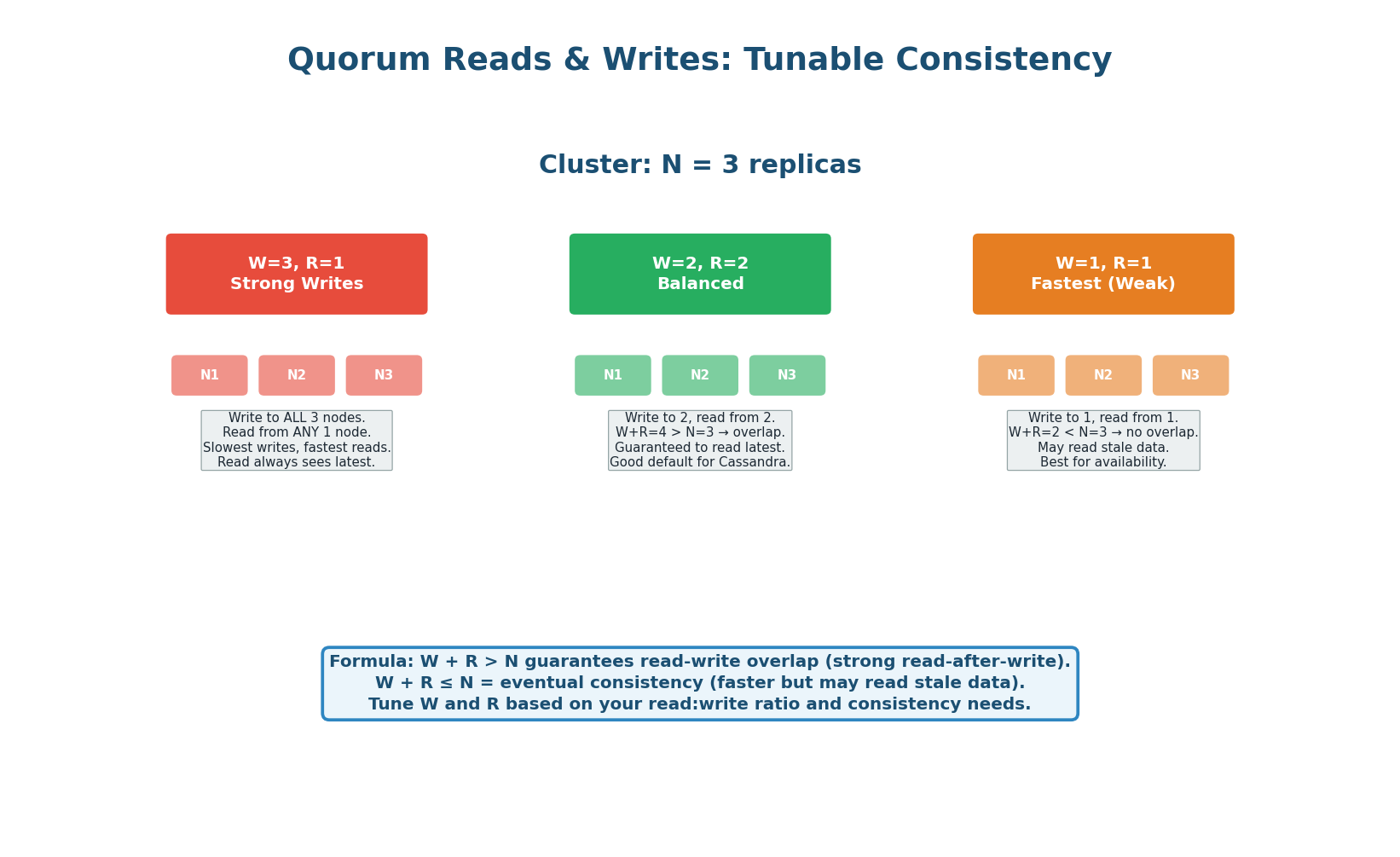
Cassandra's consistency level QUORUM sets W=⌈N/2⌉+1, R=⌈N/2⌉+1. With N=3, that's W=2, R=2 — strongly consistent and equivalent to a CP system during normal operation. Cassandra with ONE sets W=1, R=1 — eventual consistency, maximum availability. Most Cassandra deployments use different consistency levels per operation: QUORUM for writes, LOCAL_ONE for non-critical reads.
Topic 3
Failure Scenarios
A Taxonomy of What Can Go Wrong
In distributed systems, failure is not an exception — it is the norm. Google's data shows that in a cluster of 10,000 servers, on average 2–3 servers fail per day, 1 network switch fails per month, and 1 rack loses power per year. Design for failure from day one; don't bolt on resilience afterwards.
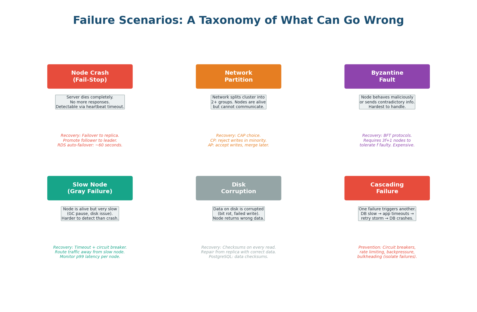
Server dies completely. Detected via heartbeat timeout (10–30s). Mitigation: automatic failover, leader re-election.
Cluster splits into isolated groups. Nodes are alive but can't communicate. The trigger for CAP trade-offs.
The most insidious. Responds but very slowly. GC pause, disk saturation, memory pressure. Circuit breakers handle this.
One failure triggers a chain. DB slow → threads block → thread pool exhausted → upstream service times out → retries amplify load.
A dead node fails fast — timeouts fire, failover kicks in. A slow node keeps responding just enough to prevent failover, but slow enough to back-pressure the entire system. Thread pools fill up waiting for the slow node. The fix: circuit breakers that detect elevated error rates or p99 latencies and temporarily stop sending traffic to the slow node, giving it time to recover.
| Failure Type | Detection | Primary Mitigation | Interview Answer |
|---|---|---|---|
| Node crash | Heartbeat timeout (10–30s) | Automatic failover, replica promotion | "We use health checks + automated failover via Pacemaker / k8s" |
| Network partition | Peer-to-peer timeout | Majority quorum (refuse minority writes) | "CAP forces a choice — we prefer CP for payment writes" |
| Slow node | p99 latency spike, timeout rate | Circuit breaker (Hystrix / Resilience4j) | "Circuit breaker opens after 5 consecutive failures, 30s recovery" |
| Cascading failure | Thread pool exhaustion, queue depth | Bulkhead isolation, backpressure, rate limiting | "Bulkhead: separate thread pools per downstream service" |
| Disk corruption | Checksum mismatch on read | Replication + checksummed storage (ZFS, ext4) | "RAID is not a substitute for replication across nodes" |
Topic 4
CAP Trade-offs
The CAP Theorem: Reframed for Interviews
The CAP theorem states that a distributed system can provide at most two of three properties: Consistency (every read returns the most recent write), Availability (every request gets a non-error response), and Partition Tolerance (the system continues operating despite network partitions).
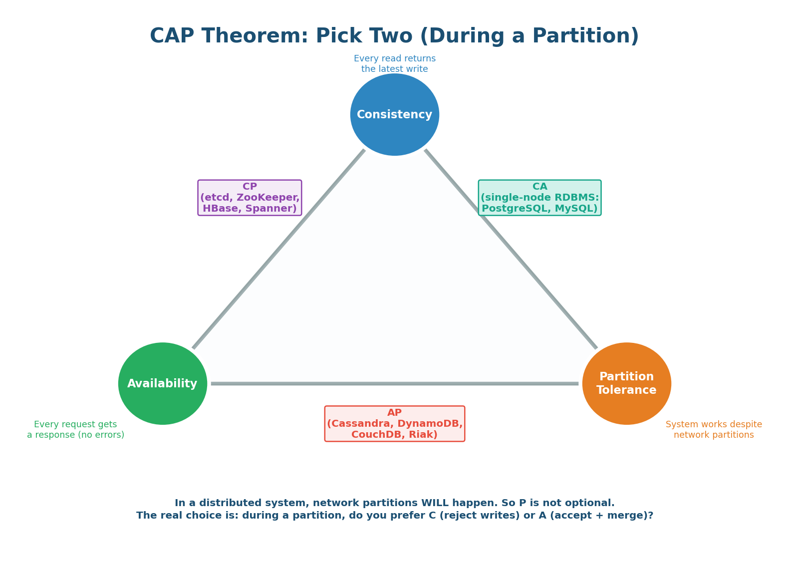
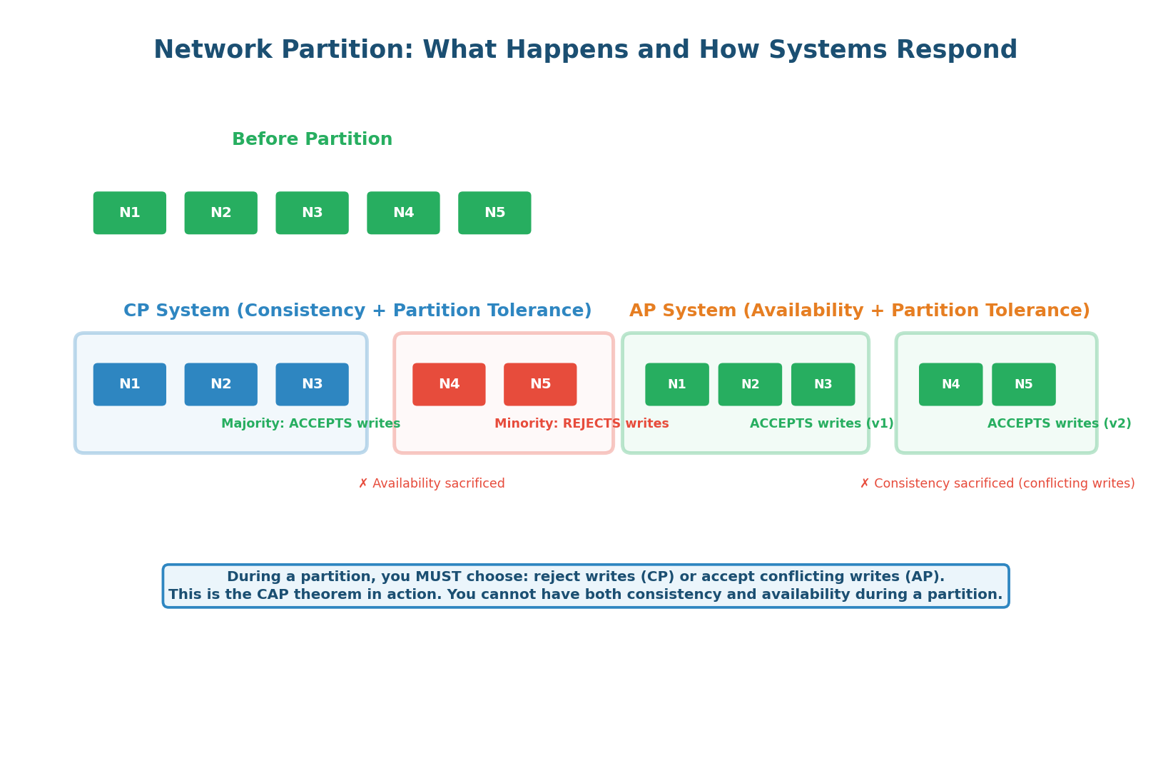
The CAP trade-off only activates when a partition occurs. During normal operation, you get all three properties. When a partition happens, you must choose: reject writes (maintain consistency, lose availability) or accept writes on both sides (maintain availability, risk inconsistency). In an interview, this is the question: "When a partition happens in your system, which do you prefer — returning an error, or returning potentially stale data?"
How Real Systems Respond to Partitions
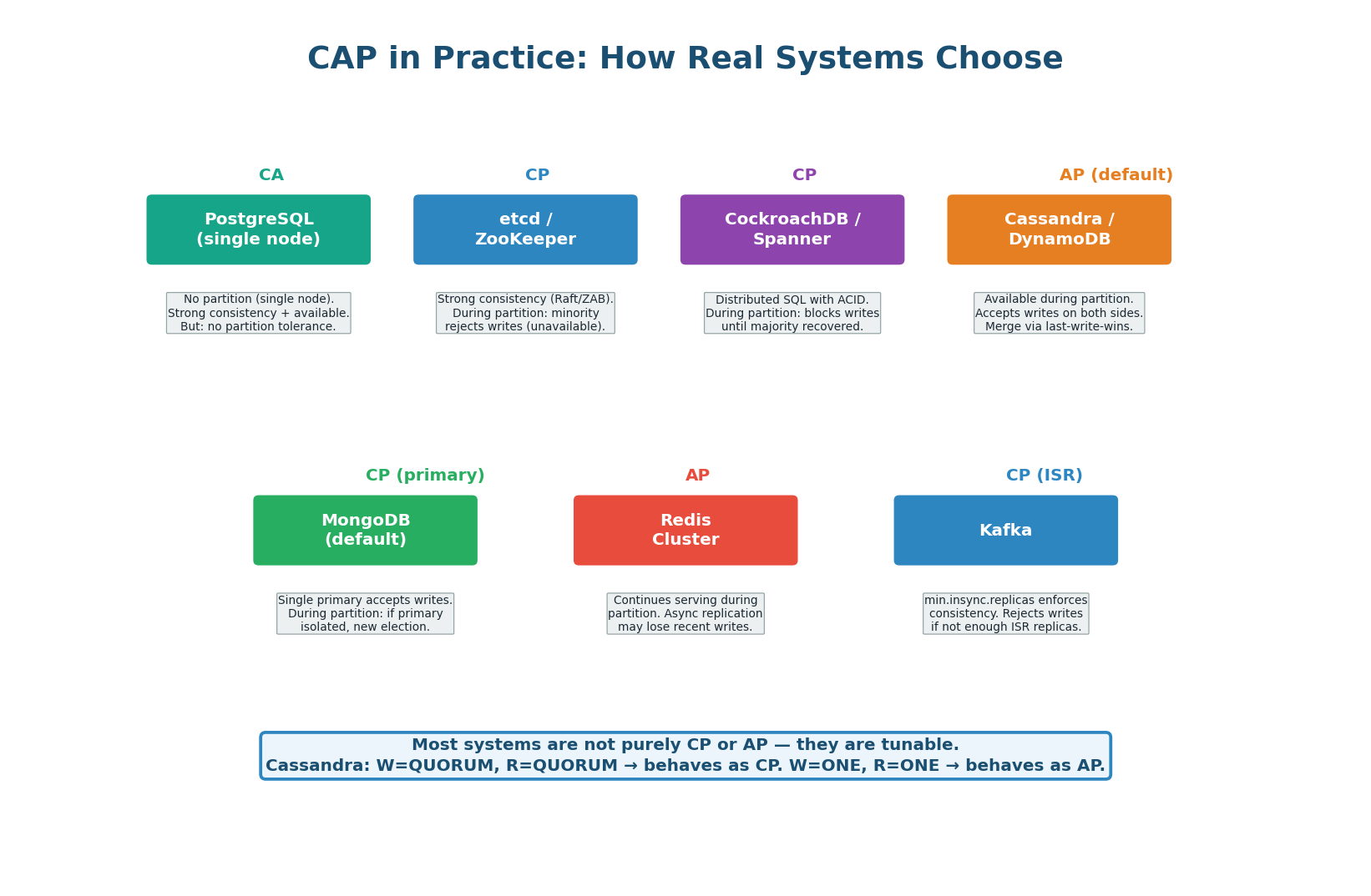
CP (Consistency + Partition tolerance): During a partition, the minority side (fewer than N/2+1 nodes) rejects all writes. Only the majority side accepts writes. This ensures no conflicting writes exist — the system is consistent. But users on the minority side get errors. etcd, ZooKeeper, and single-leader PostgreSQL with synchronous replication are CP.
AP (Availability + Partition tolerance): During a partition, BOTH sides continue accepting writes. Users on both sides get responses (no errors). But the two sides may have conflicting data — User 42's balance might be $500 on one side and $300 on the other. Once the partition heals, these conflicts must be resolved. Cassandra with ONE, DynamoDB without transactions, and DNS are AP.
| System | Default CAP Position | Tunable? | When to Choose |
|---|---|---|---|
| PostgreSQL (primary only) | CA (no partition tolerance) | Add replicas → CP | Single-region, strong consistency required |
| etcd / ZooKeeper | CP | No | Coordination (locks, leader election, config) |
| Cassandra | AP (default) | Yes — QUORUM = CP | High write throughput, eventual consistency OK |
| DynamoDB | AP (eventual reads default) | Yes — strongly consistent reads available | Scale-out key-value, tunable per read |
| CockroachDB | CP | No | Multi-region, strong consistency, SQL interface |
| MongoDB | CP (default with writeConcern majority) | Yes — lower writeConcern = AP-like | General-purpose document store |
Conflict Resolution in AP Systems
AP systems accept writes on both sides of a partition. When the partition heals, conflicting versions must be reconciled. There are three standard strategies:
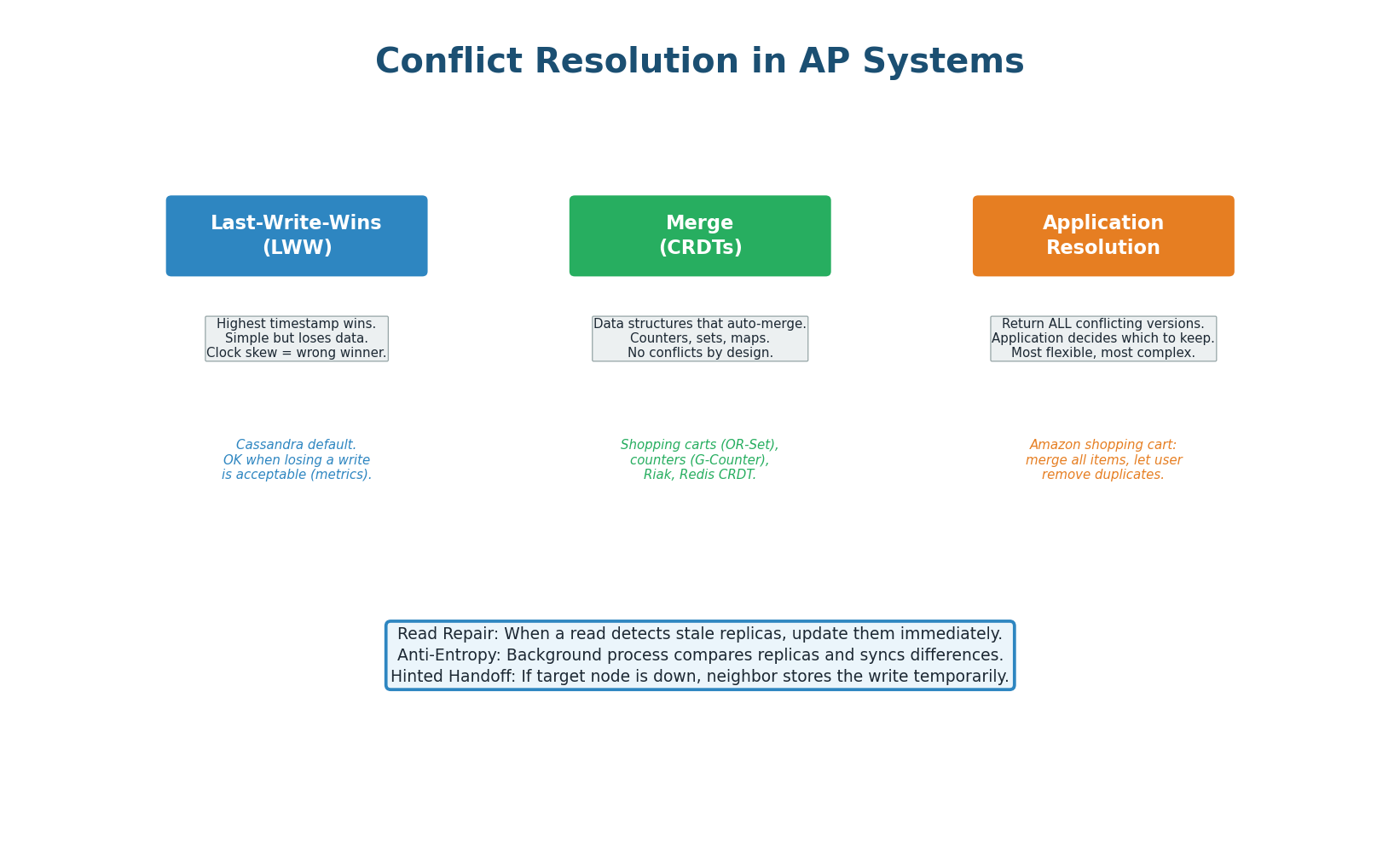
Last-Write-Wins (LWW): Compare timestamps, keep the value with the highest timestamp. Simple to implement but loses data: if two users update the same field at roughly the same time, one update is silently discarded. DynamoDB and Cassandra use LWW by default. Acceptable for use cases where the last write is semantically correct (e.g., "last viewed at" timestamp).
CRDTs (Conflict-free Replicated Data Types): Mathematical data structures designed to merge without conflicts. A G-Counter (grow-only counter) on each node independently increments, and merging takes the max of each node's counter — no data is ever lost. Shopping carts modeled as add-only sets (G-Set) can merge trivially. CRDTs only work for data types where merge is mathematically well-defined. Riak and Redis CRDT module use these.
Application-Level Resolution: The database returns all conflicting versions to the application, which decides how to merge. Amazon's original shopping cart design (DynamoDB paper): if two concurrent operations added different items to the cart, the merged cart contains both. Amazon chose to never lose an item — even at the cost of phantom items appearing. The application knows the domain semantics better than the database.
| Strategy | Data Loss Risk | Complexity | Best For |
|---|---|---|---|
| Last-Write-Wins | High (concurrent updates lost) | Low | Metadata, timestamps, idempotent writes |
| CRDTs | None (by design) | Medium (only specific data types) | Counters, sets, add-only collections |
| Application resolution | Depends on logic | High (custom per domain) | Shopping carts, collaborative editing, business-critical merges |
| Avoid conflict (CP) | None | Low (use a CP system) | Financial transactions, inventory, locks |
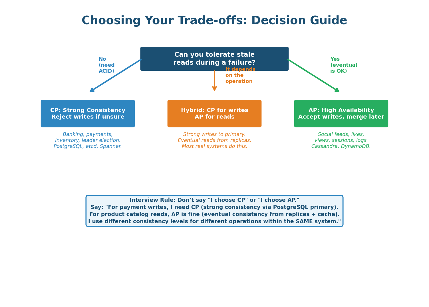
The Decision Framework
The most important takeaway from this class: you do not choose CP or AP for your entire system. You choose per-operation. Within the same application, payment writes use CP (PostgreSQL primary, strong consistency), user feed reads use AP (Cassandra eventual, fast), and session tokens use CP (Redis with quorum). The framework:
| Operation Type | CAP Choice | Why | Example |
|---|---|---|---|
| Payment, debit, inventory decrement | CP — strong consistency | Data loss or duplicate processing is catastrophic | PostgreSQL primary with synchronous replication |
| User profile read, feed, recommendations | AP — eventual consistency | Slightly stale data is invisible to users; availability matters more | Cassandra with ONE consistency |
| Distributed lock, leader election | CP — consensus-backed | Multiple processes believing they hold a lock = split-brain disaster | etcd, ZooKeeper |
| Like counts, view counters | AP — CRDTs or LWW | Exact count doesn't matter; approximate is fine | Cassandra counter column or Redis CRDT |
| Shopping cart | AP — application merge | Never lose an item; merge on conflict | DynamoDB with application-level resolution |
Class Summary
Four Topics, One Framework
Partitioning
Shard for write throughput and data capacity. Pay the price in cross-shard joins and operational complexity. Partition key choice is irreversible — get locality vs. distribution right upfront.
Replication
Single-leader (simplest, default). Multi-leader (cross-region writes, complex conflicts). Leaderless (tunable via W+R>N). Default to single-leader in interviews unless multi-region writes are explicitly required.
Failure Taxonomy
Node crash → failover. Network partition → CAP choice. Slow node → circuit breaker. Cascading → bulkhead. Gray failures (slow nodes) are more dangerous than hard crashes.
CAP Trade-offs
CAP only matters during a partition. Choose CP for financial operations and locks. Choose AP for reads, counters, and carts. Most real systems are tunable — you choose per-operation, not per-system.
Conflict Resolution
LWW (simple, lossy) → CRDTs (math-safe, limited types) → Application resolution (flexible, complex). For anything financial, avoid AP systems entirely — use CP and avoid the conflict problem.
Interview Rule
Never start with sharding. Never start with multi-leader. Start simple, scale vertically, add read replicas, then shard. Justify every complexity you introduce.
Want to Land at Google, Microsoft or Apple?
Watch Pranjal Jain's free 30-min training — the exact GROW Strategy that helped 1,572+ engineers go from TCS/Infosys to top product companies with a 3–5X salary hike.