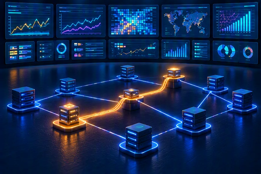
- Metrics tell you that something is wrong (cheap, aggregated, alertable). Traces tell you where (which service, which call). Logs tell you why (the exact error and context). Link them with a shared trace ID.
- Logs: structured JSON, consistent fields, trace ID in every line, never PII or secrets. Metrics: counters, gauges, histograms; keep label cardinality bounded.
- Tracing works by propagating context (W3C
traceparent) through every HTTP call and message header. OpenTelemetry gives you vendor-neutral SDKs, auto-instrumentation and a Collector. - Dashboards: RED (Rate, Errors, Duration) per service, USE (Utilization, Saturation, Errors) per resource.
- Reliability targets: SLI (what you measure) → SLO (target, e.g. 99.9% over 30 days = ~43 min of budget) → alert on error budget burn rate, not on CPU spikes.
In a monolith, a slow request means opening one log file. In a system of 40 microservices, a checkout that takes 6 seconds could be slow because of the payment gateway, a cold cache, a lock in the inventory database, a retry storm, or a noisy neighbour on one Kubernetes node. Observability is the discipline of emitting enough structured telemetry that you can answer "what is happening and why" from the outside, including for failures nobody anticipated. This guide covers how each signal works, how to wire them together with OpenTelemetry, and how to turn them into SLOs and alerts that wake people up only when users are hurting.
Monitoring vs Observability
Monitoring answers known questions: is CPU above 80%? Is the error rate above 1%? It relies on dashboards and alerts you set up in advance. Observability is a property of the system: can you ask a new question, like "are failed UPI payments concentrated on one bank, one app version and one pod?", using telemetry you already have, without deploying new code?
The practical difference is dimensionality. A metric "payment_failures_total" tells you failures went up. A trace or wide structured event with attributes (bank, PSP, app version, pod, region, merchant category) lets you slice until the pattern appears. The three pillars are different trade-offs between cost and detail:
| Metrics | Logs | Traces | |
|---|---|---|---|
| Shape | Numbers aggregated over time, with labels | Timestamped event records | Tree of timed spans per request |
| Answers | Is something wrong? How much? Trend? | What exactly happened in this event? | Where did time go across services? |
| Cost per request | ~Zero (aggregated) | Proportional to volume | High unless sampled |
| Retention | Months to years | Days to weeks (hot) | Days, sampled |
| Good for alerts | Yes | Sometimes (log-based metrics) | Rarely directly |
| Typical tools | Prometheus, Grafana Mimir, Datadog | ELK/OpenSearch, Loki, Splunk | Jaeger, Grafana Tempo, Zipkin, vendor APMs |
Logs Done Right: Structured, Correlated, Affordable
Unstructured logs like Payment failed for user 123 amount 499 are readable by humans and miserable for machines. Structured logs make every field queryable:
{
  "ts": "2026-10-09T14:03:22.418Z",
  "level": "ERROR",
  "service": "payment-service",
  "env": "prod",
  "version": "2.18.1",
  "trace_id": "4bf92f3577b34da6a3ce929d0e0e4736",
  "span_id": "00f067aa0ba902b7",
  "event": "payment.authorize.failed",
  "order_id": "ORD-88213",
  "psp": "bank_x",
  "method": "upi",
  "error_code": "U30",
  "latency_ms": 2840,
  "msg": "PSP returned debit failure"
}
Logging rules that pay off
- Use a stable event name (
payment.authorize.failed) rather than relying on free-text messages for search. - Include
trace_idandspan_idin every line; OpenTelemetry logging integrations and MDC (Java) do this automatically. This is the bridge from a trace to its logs. - Levels mean something: ERROR = needs attention, WARN = degraded but handled, INFO = business events, DEBUG = off in production or sampled.
- Never log secrets or PII: card numbers, full phone numbers, Aadhaar, OTPs, auth headers. Mask in a shared logging library; India's DPDP Act raises the stakes for personal data.
- Control volume. Log aggregation is often the largest observability bill. Sample repetitive success logs, drop health-check noise, and keep error logs at 100%.
- Write to stdout in containers and let an agent (Fluent Bit, Vector, the OTel Collector) ship them. Building that pipeline at scale is its own design problem: Design a Distributed Logging System.
Metrics: Types, Histograms and the Cardinality Trap
The four metric types
| Type | Behaviour | Example | Query with |
|---|---|---|---|
| Counter | Only goes up (resets on restart) | http_requests_total | rate() over a window |
| Gauge | Goes up and down | Queue depth, memory in use, active connections | Current value, avg_over_time |
| Histogram | Counts observations into buckets, plus sum and count | Request latency | histogram_quantile() |
| Summary | Client-computed quantiles | Latency p99 per instance | Cannot be aggregated across instances |
Prefer histograms over summaries for latency: you can aggregate buckets across 30 pods and then compute a fleet-wide p99. Averaging per-pod p99s is mathematically meaningless.
# Rate: requests per second, by route
sum by (http_route) (rate(http_server_request_duration_seconds_count{service="checkout"}[5m]))

# Errors: fraction of 5xx responses
sum(rate(http_server_request_duration_seconds_count{service="checkout", http_response_status_code=~"5.."}[5m]))
  /
sum(rate(http_server_request_duration_seconds_count{service="checkout"}[5m]))

# Duration: fleet-wide p99 latency from histogram buckets
histogram_quantile(0.99,
  sum by (le) (rate(http_server_request_duration_seconds_bucket{service="checkout"}[5m])))
Cardinality: the most expensive mistake in metrics
Each unique combination of label values is a separate time series. http_requests_total{route, method, status} with 50 routes × 4 methods × 10 status codes = 2,000 series per instance; fine. Add user_id with 10 million users and you have created a time series database outage. Bounded labels only: route templates (/orders/{id}, not /orders/88213), status class, region, version. Put unbounded identifiers in logs and span attributes. How a metrics backend stores and downsamples these series is covered in Design a Metrics Monitoring & Alerting System.
Distributed Tracing: Spans, Trees and Waterfalls
A trace represents one request's journey. It is a tree of spans; each span is one unit of work with a name, start time, duration, status, attributes, and the ID of its parent span.
The waterfall makes the culprit obvious in seconds: the payment gateway timed out at 2 s and the retry succeeded. Without the trace, you would see "checkout p99 = 3.1 s" on a dashboard and start guessing. Traces also expose sequential calls that should be parallel (cart and pricing above could overlap), N+1 queries (200 identical DB spans in one request), and retry amplification.
How Trace Context Propagates Across Services
For spans in different processes to join one trace, each outgoing call must carry the trace ID and the caller's span ID. The standard is the W3C Trace Context traceparent header:
traceparent: 00-4bf92f3577b34da6a3ce929d0e0e4736-00f067aa0ba902b7-01
             │  │                                │                │
             │  trace-id (16 bytes, hex)         parent span-id   flags (01 = sampled)
version- Ingress: the first service (or gateway) finds no
traceparent, creates a new trace ID and root span. - Outgoing HTTP/gRPC: the instrumentation injects
traceparent(and optionaltracestate,baggage) into request headers, with the current span as parent. - Receiving service: extracts the header and starts a child span with the same trace ID.
- Async messaging: the producer injects the context into Kafka record headers or SQS message attributes; the consumer extracts it and creates a span linked to (or a child of) the producer span.
- Thread hops: inside a process, context lives in thread-local or async-context storage. Thread pools and reactive code need context-aware executors, or the trace breaks.
from opentelemetry import trace
from opentelemetry.propagate import inject, extract

tracer = trace.get_tracer("order-events")

def publish(producer, topic, key, value):
    with tracer.start_as_current_span("order.publish", kind=trace.SpanKind.PRODUCER):
        carrier = {}
        inject(carrier)                                   # writes traceparent into dict
        headers = [(k, v.encode()) for k, v in carrier.items()]
        producer.send(topic, key=key, value=value, headers=headers)

def consume(record, handle):
    carrier = {k: v.decode() for k, v in (record.headers or [])}
    ctx = extract(carrier)                                # rebuild parent context
    with tracer.start_as_current_span("order.process", context=ctx,
                                      kind=trace.SpanKind.CONSUMER):
handle(record.value)OpenTelemetry in Practice
OpenTelemetry (OTel) is the CNCF standard that merged OpenTracing and OpenCensus. It defines APIs and SDKs per language, semantic conventions (standard attribute names like http.route, db.system), the OTLP protocol, and the Collector, a pipeline that receives, processes and exports telemetry.
Zero-code instrumentation for Java
java -javaagent:/otel/opentelemetry-javaagent.jar \
     -Dotel.service.name=checkout-service \
     -Dotel.exporter.otlp.endpoint=http://otel-collector:4317 \
     -Dotel.exporter.otlp.protocol=grpc \
     -jar checkout.jar
The Java agent automatically instruments common libraries (Spring MVC, JDBC, Kafka clients, gRPC, many HTTP clients), producing spans and RED metrics with no code changes. Add manual spans for business logic.
from opentelemetry import trace
from opentelemetry.sdk.resources import Resource
from opentelemetry.sdk.trace import TracerProvider
from opentelemetry.sdk.trace.export import BatchSpanProcessor
from opentelemetry.exporter.otlp.proto.grpc.trace_exporter import OTLPSpanExporter

provider = TracerProvider(resource=Resource.create({
    "service.name": "payment-service", "deployment.environment": "prod"}))
provider.add_span_processor(BatchSpanProcessor(
    OTLPSpanExporter(endpoint="otel-collector:4317", insecure=True)))
trace.set_tracer_provider(provider)
tracer = trace.get_tracer(__name__)

def authorize(order, psp_client):
    with tracer.start_as_current_span("payment.authorize") as span:
        span.set_attribute("payment.method", order.method)   # bounded values only
        span.set_attribute("payment.psp", psp_client.name)
        try:
            return psp_client.authorize(order)
        except Exception as exc:
            span.record_exception(exc)
            span.set_status(trace.Status(trace.StatusCode.ERROR))
            raise
Sampling
- Head sampling (decide at the root, e.g.
parentbased_traceidratioat 5%): cheap, consistent across services, but may discard the one slow request you need. - Tail sampling (in the Collector, after the trace completes): keep 100% of errors and requests above 2 s, plus 1–5% of the rest. Better signal; needs all spans of a trace routed to the same Collector instance (load balance by trace ID).
RED, USE and the Four Golden Signals
Rate, Errors, Duration
For every request-driven service and endpoint: requests/s, failed requests/s (or ratio), latency distribution (p50, p95, p99). This is the first row of every service dashboard.
Utilization, Saturation, Errors
For every resource: CPU, memory, disk, network, connection pools, thread pools, Kafka consumer lag. Saturation (queue length, wait time) predicts trouble before utilization hits 100%.
Four golden signals
Latency, traffic, errors, saturation. Essentially RED plus saturation; useful as the minimum set for user-facing systems.
A practical layout: top row is RED for the user journey (checkout success rate, latency); second row is RED per dependency (payment, inventory, pricing); third row is USE for the service's resources (CPU throttling, heap, DB pool wait time, consumer lag). Separate latency of successful and failed requests; fast failures can make average latency look great during an outage.
SLIs, SLOs and Error Budgets (with the Math)
- SLI (indicator): a ratio of good events to valid events. "Proportion of checkout requests that return a non-5xx response within 1 second."
- SLO (objective): target for the SLI over a window. "99.9% over a rolling 30 days."
- SLA (agreement): a contractual promise with penalties, usually looser than the internal SLO.
- Error budget: 1 − SLO. The allowed amount of badness.
| SLO | Budget | Full downtime allowed per 30 days | Failed requests allowed at 100M requests/month |
|---|---|---|---|
| 99% | 1% | 7.2 hours | 1,000,000 |
| 99.5% | 0.5% | 3.6 hours | 500,000 |
| 99.9% | 0.1% | 43.2 minutes | 100,000 |
| 99.95% | 0.05% | 21.6 minutes | 50,000 |
| 99.99% | 0.01% | 4.32 minutes | 10,000 |
(30 days = 43,200 minutes; 0.1% of that is 43.2.) Each extra nine costs disproportionately more engineering. Also note that your SLO cannot exceed the product of your hard dependencies' availability unless you add redundancy: three serial dependencies at 99.9% each give at most about 99.7%.
Alert on burn rate, not on symptoms of symptoms
Burn rate = observed error rate ÷ budgeted error rate. Burn rate 1 spends exactly the budget over the window. The Google SRE Workbook suggests multi-window alerts such as:
| Severity | Burn rate | Long window / short window | Budget consumed if sustained |
|---|---|---|---|
| Page | 14.4 | 1 hour / 5 minutes | 2% of 30-day budget in 1 hour |
| Page | 6 | 6 hours / 30 minutes | 5% in 6 hours |
| Ticket | 1 | 3 days / 6 hours | 10% in 3 days |
For a 99.9% SLO, burn rate 14.4 means an error rate of 1.44%. Requiring both the long and short windows to exceed the threshold means the alert fires quickly on a real incident and stops quickly after recovery. Compare that to "alert if CPU > 80%", which pages people at 3 AM for a batch job that harms nobody.
Putting It Together: A Checkout Latency Incident
- Alert fires: checkout latency SLO burn rate 14× over 1 h and 5 min. (Metrics)
- Dashboard: checkout p99 jumped from 600 ms to 3.2 s at 19:42. Error rate is normal, so it is slowness, not failure. Per-dependency RED shows payment-service p99 up; inventory and pricing flat. (Metrics)
- Exemplars / trace search: open slow traces from that window; waterfalls show first PSP attempt timing out at 2 s, then a retry succeeding. (Traces)
- Slice by attributes: slow spans all have
payment.psp = bank_x. (Traces) - Jump to logs by trace ID:
psp_clientlogs show connection timeouts to one PSP endpoint IP. (Logs) - Mitigate: route traffic for that PSP to a backup, lower the timeout, open the circuit breaker. Write the postmortem with the timeline reconstructed from telemetry.
Metrics found it, traces located it, logs explained it. The mitigation step depends on resilience patterns being in place; see Circuit Breaker, Retries & Backoff.
How Observability Comes Up in Interviews
In system design rounds, interviewers increasingly ask "how would you know this is working?" near the end. Strong candidates name concrete SLIs for the design, not just "add monitoring". For a ride-hailing app: match success rate within 30 s, ETA error, location update lag. For a payment system: authorization success rate by PSP, p99 latency, reconciliation mismatches. For a Kafka pipeline: consumer lag in seconds.
Questions you should be ready for
- "How does a trace ID get from service A to service C through Kafka?" (inject/extract into headers; W3C
traceparent) - "Why is averaging p99 across pods wrong, and what do you do instead?" (aggregate histogram buckets)
- "Our Prometheus is running out of memory." (cardinality: find the label explosion with
topkon series counts per metric) - "What SLO would you set and how would you alert?" (SLI definition, window, burn-rate alerts)
- "Logs are costing too much. What do you cut?" (sampling successes, dropping debug, shorter hot retention, moving to object storage tiers)
- "How do you monitor a system where the failure is silent, like dropped notifications?" (end-to-end synthetic probes, reconciliation counts between producer and consumer)
Observability questions also appear in microservices interview questions, and running the stack on Kubernetes ties back to Docker & Kubernetes for Backend Engineers.
Frequently Asked Questions
Master System Design Interviews
Prepflix's system design course teaches you to discuss monitoring, SLOs and failure handling the way senior engineers do in real design reviews.
Explore the Prepflix Course →